Outline Control structure design plantwide control A procedure

Outline • Control structure design (plantwide control) • A procedure for control structure design I Top Down • • Step 1: Degrees of freedom Step 2: Operational objectives (optimal operation) Step 3: What to control ? (self-optimizing control) Step 4: Where set production rate? II Bottom Up • Step 5: Regulatory control: What more to control ? • Step 6: Supervisory control • Step 7: Real-time optimization • Case studies 1

II. Bottom-up • Determine secondary controlled variables and structure (configuration) of control system (pairing) • A good control configuration is insensitive to parameter changes Step 5. REGULATORY CONTROL LAYER 5. 1 Stabilization (including level control) 5. 2 Local disturbance rejection (inner cascades) What more to control? (secondary variables) Step 6. SUPERVISORY CONTROL LAYER Decentralized or multivariable control (MPC)? Pairing? Step 7. OPTIMIZATION LAYER (RTO) 2

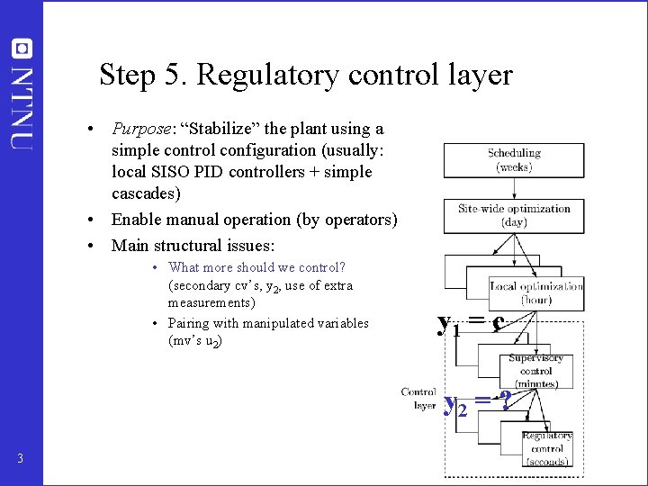
Step 5. Regulatory control layer • Purpose: “Stabilize” the plant using a simple control configuration (usually: local SISO PID controllers + simple cascades) • Enable manual operation (by operators) • Main structural issues: • What more should we control? (secondary cv’s, y 2, use of extra measurements) • Pairing with manipulated variables (mv’s u 2) y 1 = c y 2 = ? 3

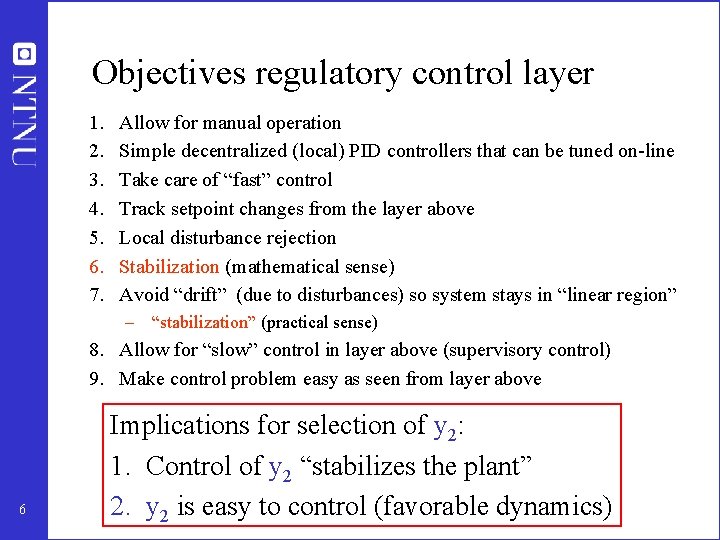
Objectives regulatory control layer 1. 2. 3. 4. 5. 6. 7. Allow for manual operation Simple decentralized (local) PID controllers that can be tuned on-line Take care of “fast” control Track setpoint changes from the layer above Local disturbance rejection Stabilization (mathematical sense) Avoid “drift” (due to disturbances) so system stays in “linear region” – “stabilization” (practical sense) 8. Allow for “slow” control in layer above (supervisory control) 9. Make control problem easy as seen from layer above The key decisions here (to be made by the control engineer) are: 1. Which extra secondary (dynamic) variables y 2 should we control? 2. Propose a (simple) control configuration (select input-output pairings) 5

Objectives regulatory control layer 1. 2. 3. 4. 5. 6. 7. Allow for manual operation Simple decentralized (local) PID controllers that can be tuned on-line Take care of “fast” control Track setpoint changes from the layer above Local disturbance rejection Stabilization (mathematical sense) Avoid “drift” (due to disturbances) so system stays in “linear region” – “stabilization” (practical sense) 8. Allow for “slow” control in layer above (supervisory control) 9. Make control problem easy as seen from layer above 6 Implications for selection of y 2: 1. Control of y 2 “stabilizes the plant” 2. y 2 is easy to control (favorable dynamics)

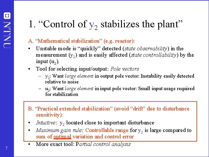
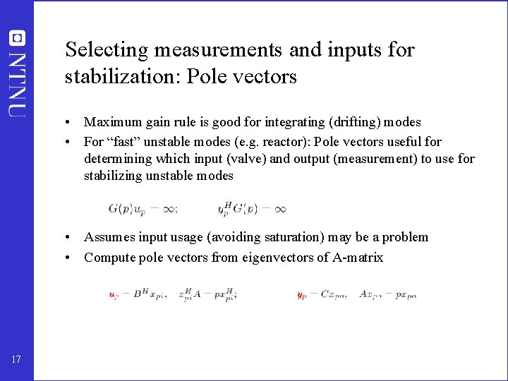
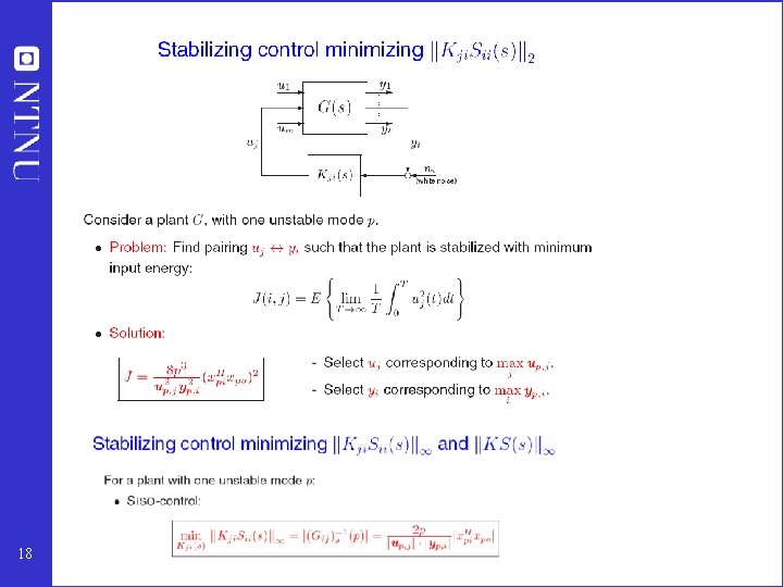
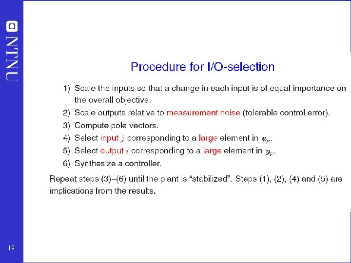
1. “Control of y 2 stabilizes the plant” A. “Mathematical stabilization” (e. g. reactor): • Unstable mode is “quickly” detected (state observability) in the measurement (y 2) and is easily affected (state controllability) by the input (u 2). • Tool for selecting input/output: Pole vectors – y 2: Want large element in output pole vector: Instability easily detected relative to noise – u 2: Want large element in input pole vector: Small input usage required for stabilization 7 B. “Practical extended stabilization” (avoid “drift” due to disturbance sensitivity): • Intuitive: y 2 located close to important disturbance • Maximum gain rule: Controllable range for y 2 is large compared to sum of optimal variation and control error • More exact tool: Partial control analysis

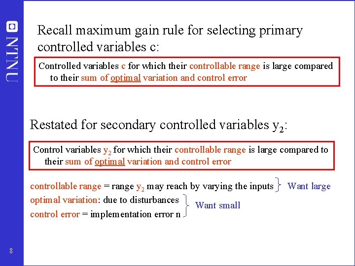
Recall maximum gain rule for selecting primary controlled variables c: Controlled variables c for which their controllable range is large compared to their sum of optimal variation and control error Restated for secondary controlled variables y 2: Control variables y 2 for which their controllable range is large compared to their sum of optimal variation and control error controllable range = range y 2 may reach by varying the inputs optimal variation: due to disturbances Want small control error = implementation error n 8 Want large

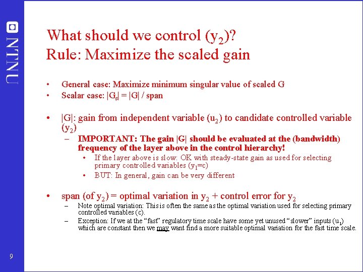
What should we control (y 2)? Rule: Maximize the scaled gain • • General case: Maximize minimum singular value of scaled G Scalar case: |Gs| = |G| / span • |G|: gain from independent variable (u 2) to candidate controlled variable (y 2) – IMPORTANT: The gain |G| should be evaluated at the (bandwidth) frequency of the layer above in the control hierarchy! • • • span (of y 2) = optimal variation in y 2 + control error for y 2 – – 9 If the layer above is slow: OK with steady-state gain as used for selecting primary controlled variables (y 1=c) BUT: In general, gain can be very different Note optimal variation: This is often the same as the optimal variation used for selecting primary controlled variables (c). Exception: If we at the “fast” regulatory time scale have some yet unused “slower” inputs (u 1) which are constant then we may want find a more suitable optimal variation for the fast time scale.

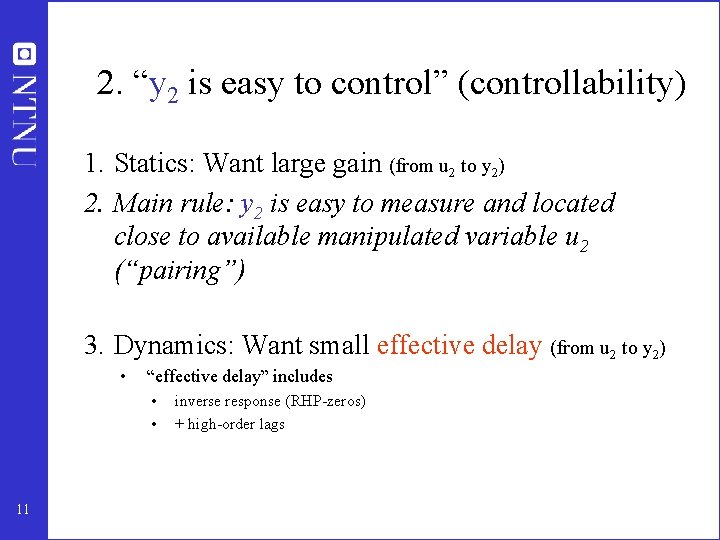
2. “y 2 is easy to control” (controllability) 1. Statics: Want large gain (from u 2 to y 2) 2. Main rule: y 2 is easy to measure and located close to available manipulated variable u 2 (“pairing”) 3. Dynamics: Want small effective delay (from u 2 to y 2) • “effective delay” includes • • 11 inverse response (RHP-zeros) + high-order lags

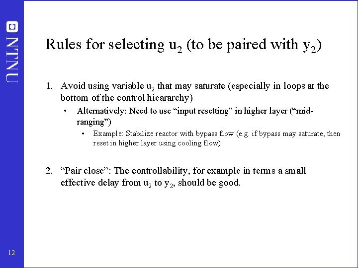
Rules for selecting u 2 (to be paired with y 2) 1. Avoid using variable u 2 that may saturate (especially in loops at the bottom of the control hieararchy) • Alternatively: Need to use “input resetting” in higher layer (“midranging”) • Example: Stabilize reactor with bypass flow (e. g. if bypass may saturate, then reset in higher layer using cooling flow) 2. “Pair close”: The controllability, for example in terms a small effective delay from u 2 to y 2, should be good. 12

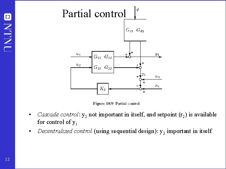
Partial control • Cascade control: y 2 not important in itself, and setpoint (r 2) is available for control of y 1 • Decentralized control (using sequential design): y 2 important in itself 13

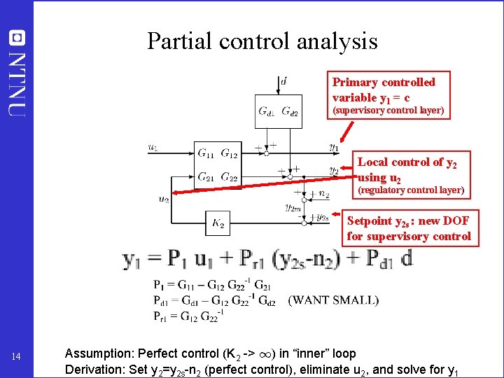
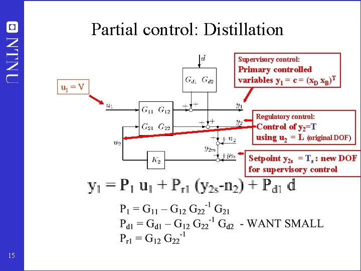
Partial control analysis Primary controlled variable y 1 = c (supervisory control layer) Local control of y 2 using u 2 (regulatory control layer) Setpoint y 2 s : new DOF for supervisory control 14 Assumption: Perfect control (K 2 -> 1) in “inner” loop Derivation: Set y 2=y 2 s-n 2 (perfect control), eliminate u 2, and solve for y 1

Partial control: Distillation Supervisory control: u 1 = V Primary controlled variables y 1 = c = (x. D x. B)T Regulatory control: Control of y 2=T using u 2 = L (original DOF) Setpoint y 2 s = Ts : new DOF for supervisory control 15

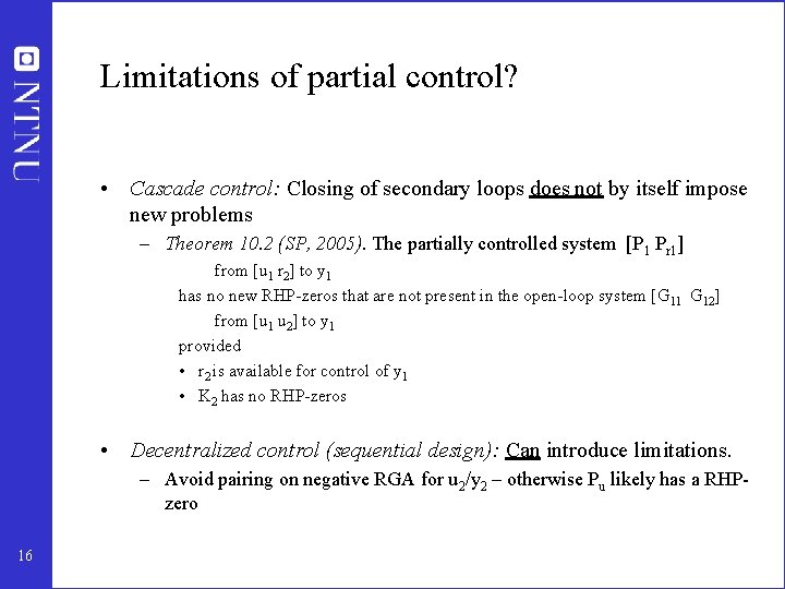
Limitations of partial control? • Cascade control: Closing of secondary loops does not by itself impose new problems – Theorem 10. 2 (SP, 2005). The partially controlled system [P 1 Pr 1] from [u 1 r 2] to y 1 has no new RHP-zeros that are not present in the open-loop system [G 11 G 12] from [u 1 u 2] to y 1 provided • r 2 is available for control of y 1 • K 2 has no RHP-zeros • Decentralized control (sequential design): Can introduce limitations. – Avoid pairing on negative RGA for u 2/y 2 – otherwise Pu likely has a RHPzero 16

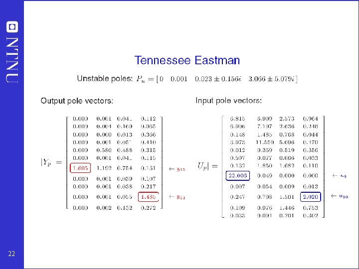
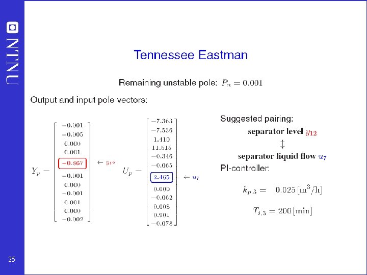
Selecting measurements and inputs for stabilization: Pole vectors • Maximum gain rule is good for integrating (drifting) modes • For “fast” unstable modes (e. g. reactor): Pole vectors useful for determining which input (valve) and output (measurement) to use for stabilizing unstable modes • Assumes input usage (avoiding saturation) may be a problem • Compute pole vectors from eigenvectors of A-matrix 17

18

19

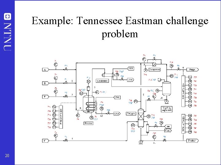
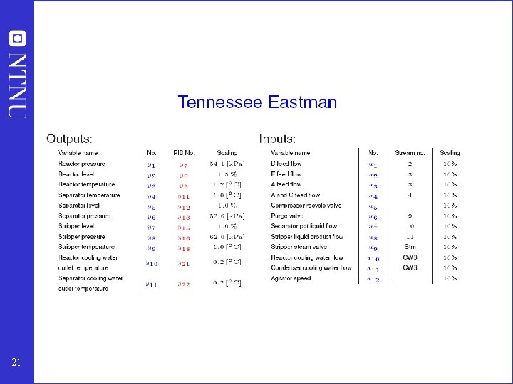
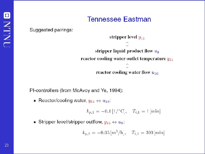
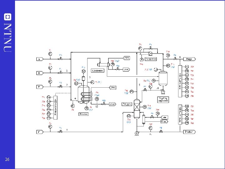
Example: Tennessee Eastman challenge problem 20

21

22

23

24

25

26