Outline by Lecture 1 Probability 90 min Definition

Outline by Lecture 1 Probability (90 min. ) Definition, Bayes’ theorem, probability densities and their properties, catalogue of pdfs, Monte Carlo 2 Statistical tests (90 min. ) general concepts, test statistics, multivariate methods, goodness-of-fit tests 3 Parameter estimation (90 min. ) general concepts, maximum likelihood, variance of estimators, least squares 4 Interval estimation (60 min. ) setting limits 5 Further topics (60 min. ) systematic errors, MCMC

Some statistics books, papers, etc.

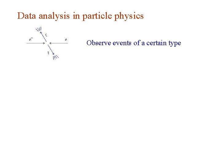
Data analysis in particle physics Observe events of a certain type

Dealing with uncertainty In particle physics there are various elements of uncertainty: theory is not deterministic quantum mechanics random measurement errors present even without quantum effects things we could know in principle but don’t e. g. from limitations of cost, time, . . . We can quantify the uncertainty using PROBABILITY

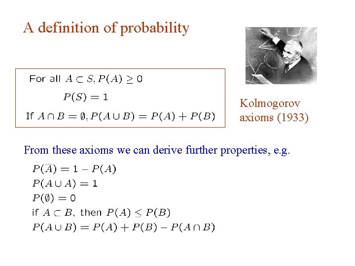
A definition of probability Kolmogorov axioms (1933) From these axioms we can derive further properties, e. g.

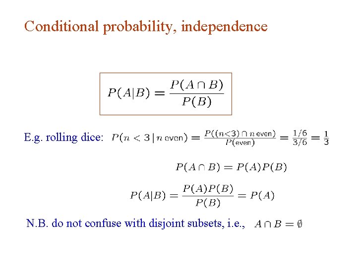
Conditional probability, independence E. g. rolling dice: N. B. do not confuse with disjoint subsets, i. e. ,

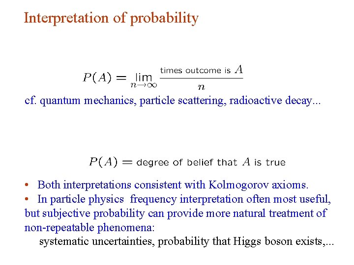
Interpretation of probability cf. quantum mechanics, particle scattering, radioactive decay. . . • Both interpretations consistent with Kolmogorov axioms. • In particle physics frequency interpretation often most useful, but subjective probability can provide more natural treatment of non-repeatable phenomena: systematic uncertainties, probability that Higgs boson exists, . . .

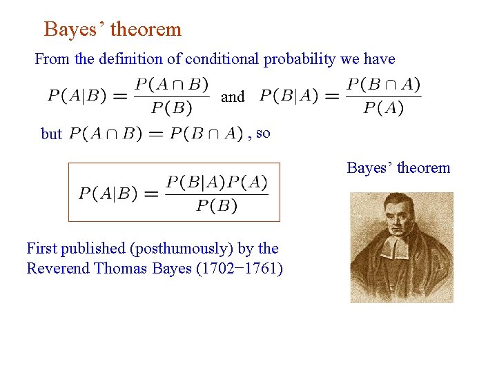
Bayes’ theorem From the definition of conditional probability we have and but , so Bayes’ theorem First published (posthumously) by the Reverend Thomas Bayes (1702− 1761)

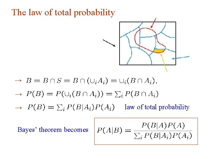
The law of total probability → → → Bayes’ theorem becomes law of total probability

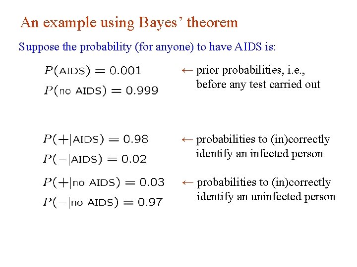
An example using Bayes’ theorem Suppose the probability (for anyone) to have AIDS is: ← prior probabilities, i. e. , before any test carried out ← probabilities to (in)correctly identify an infected person ← probabilities to (in)correctly identify an uninfected person

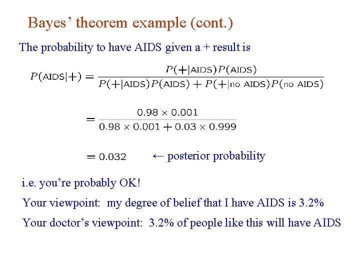
Bayes’ theorem example (cont. ) The probability to have AIDS given a + result is ← posterior probability i. e. you’re probably OK! Your viewpoint: my degree of belief that I have AIDS is 3. 2% Your doctor’s viewpoint: 3. 2% of people like this will have AIDS

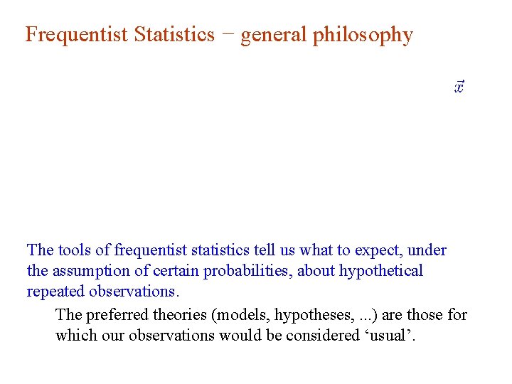
Frequentist Statistics − general philosophy The tools of frequentist statistics tell us what to expect, under the assumption of certain probabilities, about hypothetical repeated observations. The preferred theories (models, hypotheses, . . . ) are those for which our observations would be considered ‘usual’.

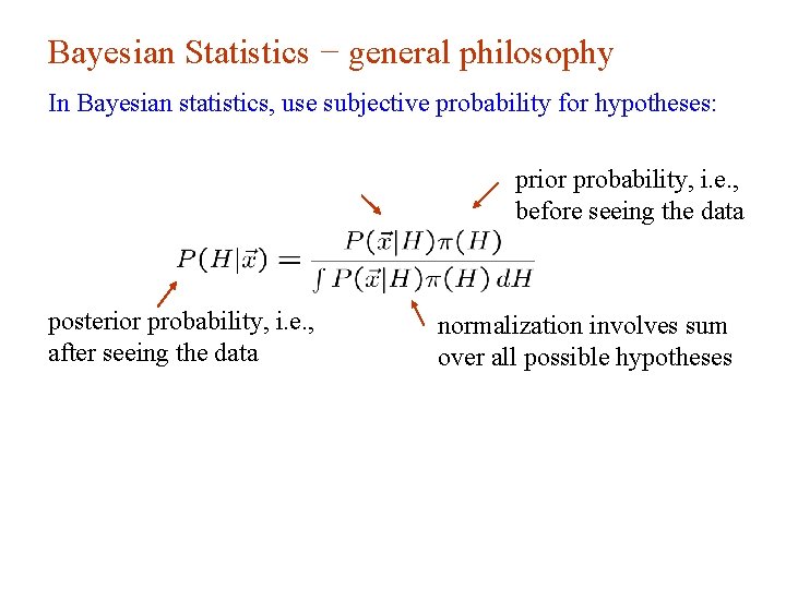
Bayesian Statistics − general philosophy In Bayesian statistics, use subjective probability for hypotheses: prior probability, i. e. , before seeing the data posterior probability, i. e. , after seeing the data normalization involves sum over all possible hypotheses

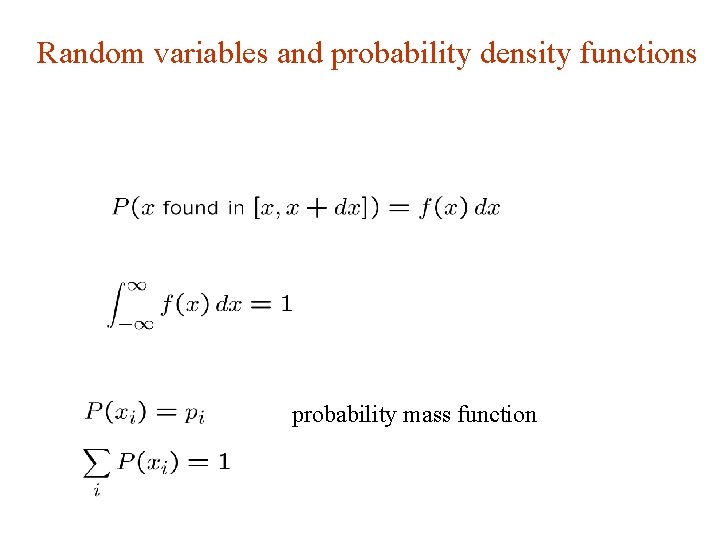
Random variables and probability density functions probability mass function

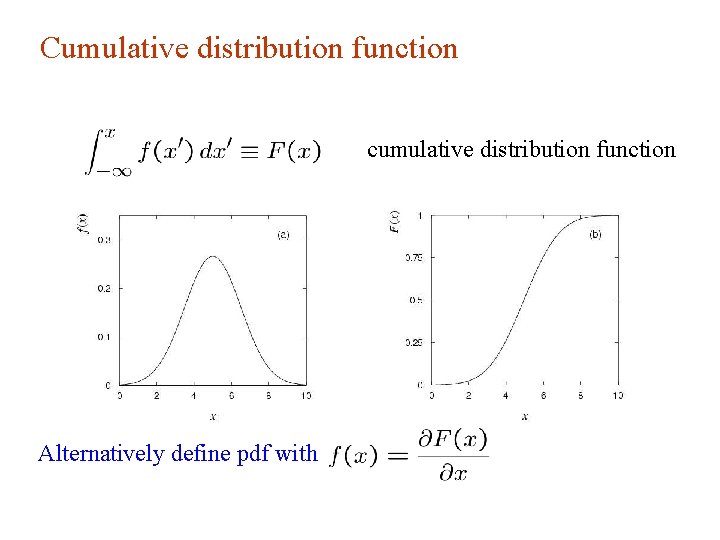
Cumulative distribution function cumulative distribution function Alternatively define pdf with

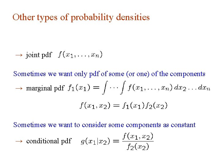
Other types of probability densities → joint pdf Sometimes we want only pdf of some (or one) of the components → marginal pdf Sometimes we want to consider some components as constant → conditional pdf

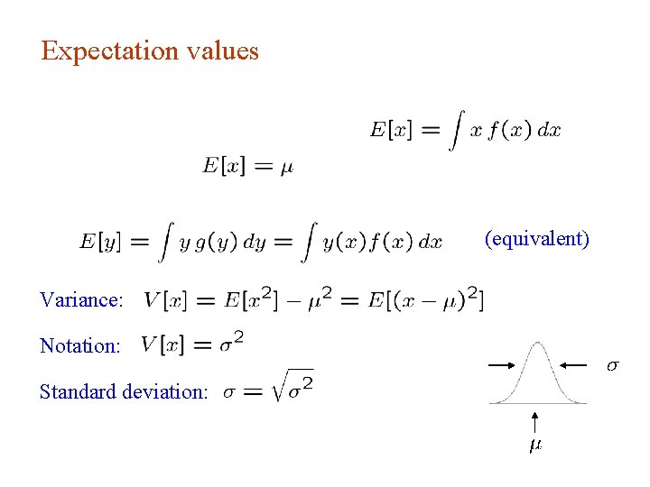
Expectation values (equivalent) Variance: Notation: Standard deviation:

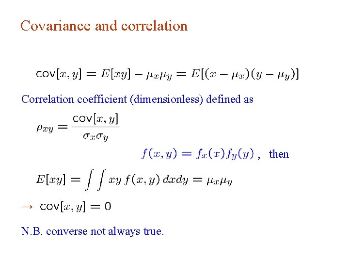
Covariance and correlation Correlation coefficient (dimensionless) defined as , then → N. B. converse not always true.

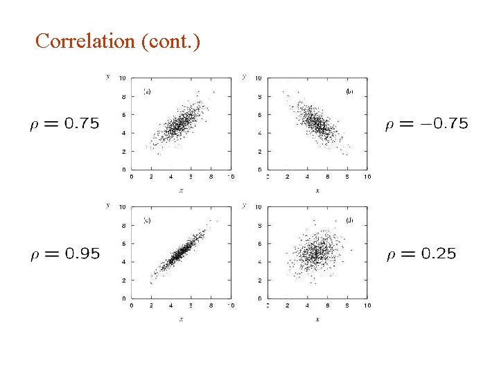
Correlation (cont. )

Some distributions

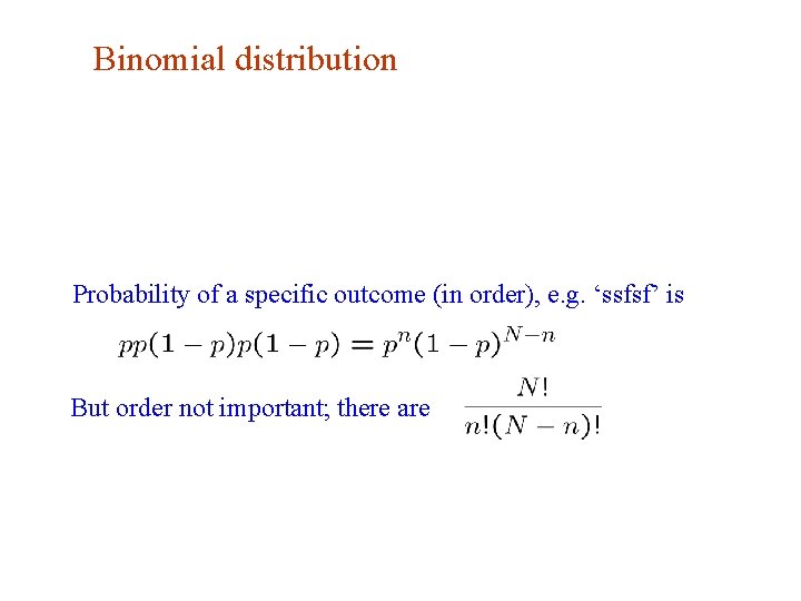
Binomial distribution Probability of a specific outcome (in order), e. g. ‘ssfsf’ is But order not important; there are

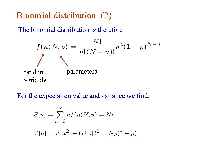
Binomial distribution (2) The binomial distribution is therefore random variable parameters For the expectation value and variance we find:

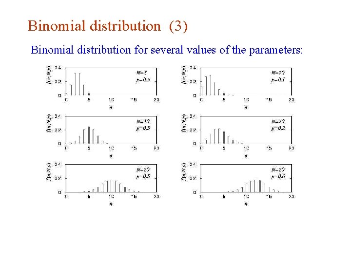
Binomial distribution (3) Binomial distribution for several values of the parameters:

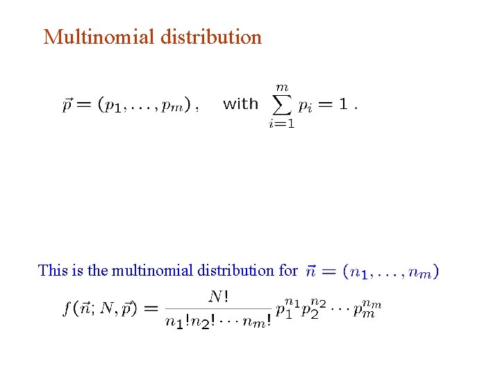
Multinomial distribution This is the multinomial distribution for

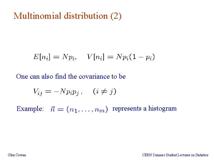
Multinomial distribution (2) One can also find the covariance to be Example: Glen Cowan represents a histogram CERN Summer Student Lectures on Statistics

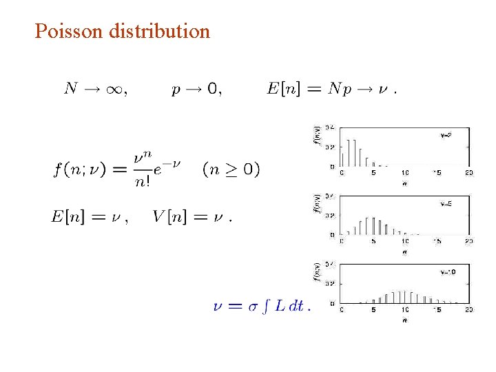
Poisson distribution

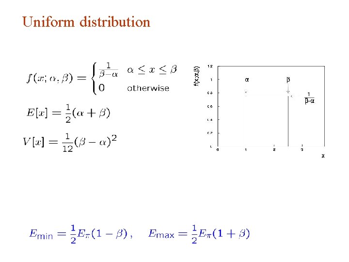
Uniform distribution

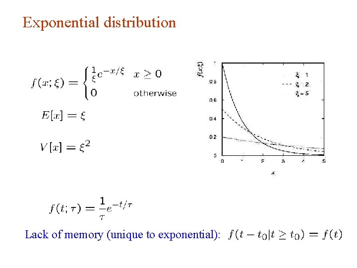
Exponential distribution Lack of memory (unique to exponential):

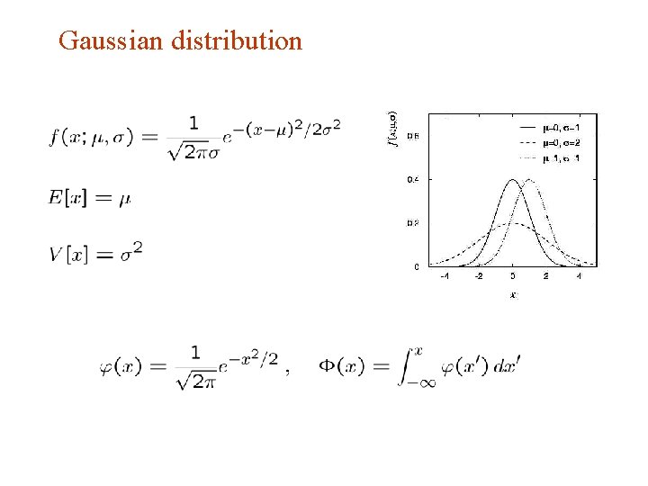
Gaussian distribution

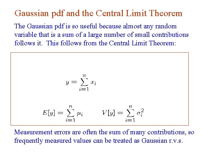
Gaussian pdf and the Central Limit Theorem The Gaussian pdf is so useful because almost any random variable that is a sum of a large number of small contributions follows it. This follows from the Central Limit Theorem: Measurement errors are often the sum of many contributions, so frequently measured values can be treated as Gaussian r. v. s.

Central Limit Theorem (2) The CLT can be proved using characteristic functions (Fourier transforms), see, e. g. , SDA Chapter 10. Beware of measurement errors with non-Gaussian tails.

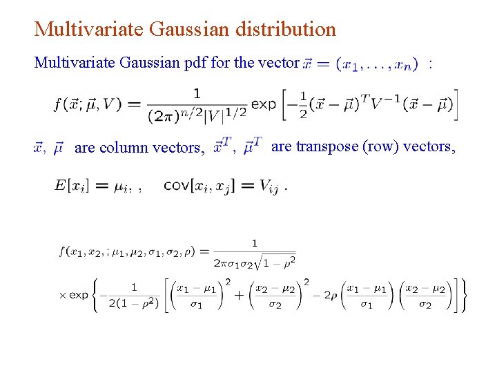
Multivariate Gaussian distribution Multivariate Gaussian pdf for the vector are column vectors, are transpose (row) vectors,

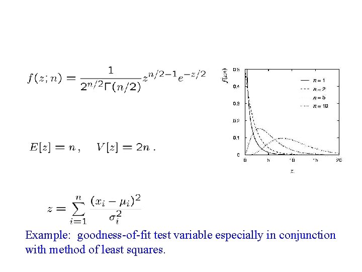
Example: goodness-of-fit test variable especially in conjunction with method of least squares.

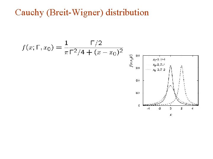
Cauchy (Breit-Wigner) distribution

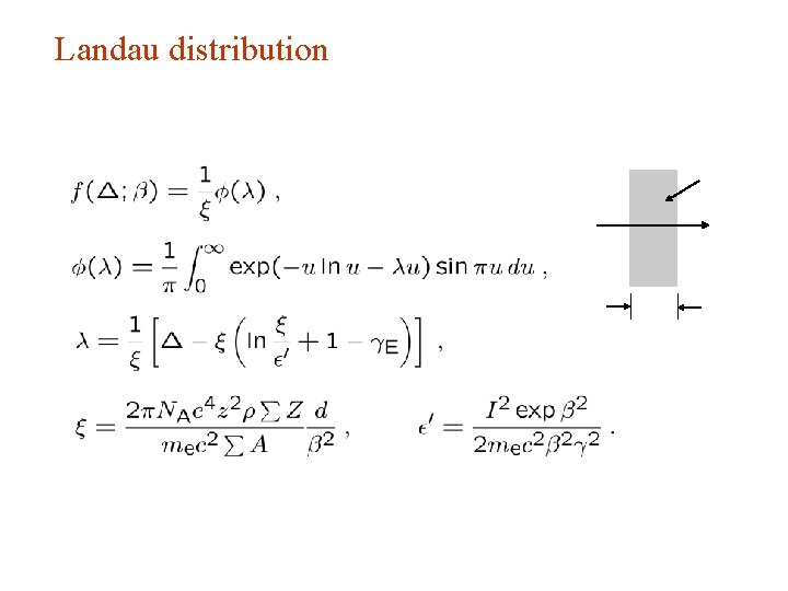
Landau distribution

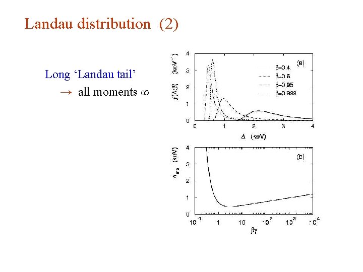
Landau distribution (2) Long ‘Landau tail’ → all moments ∞

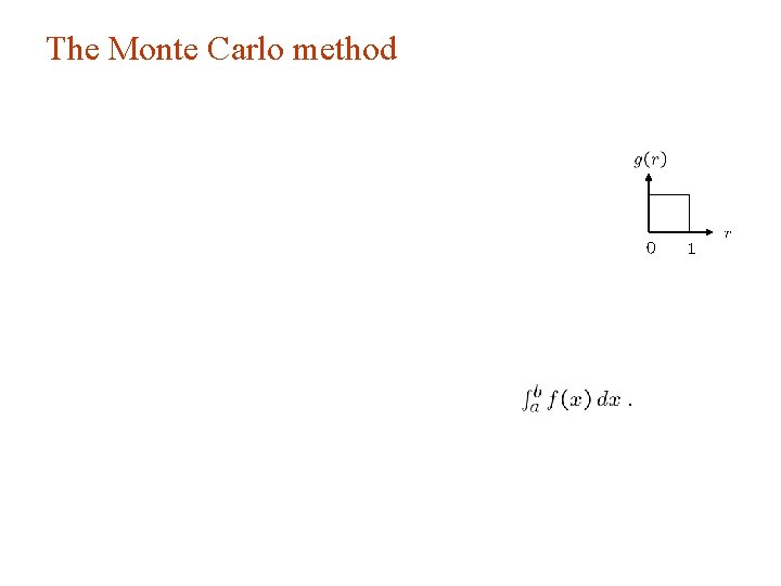
The Monte Carlo method

Random number generators

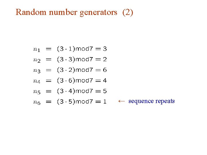
Random number generators (2) ← sequence repeats

Random number generators (3) are in [0, 1] but are they ‘random’? See F. James, Comp. Phys. Comm. 60 (1990) 111; Brandt Ch. 4

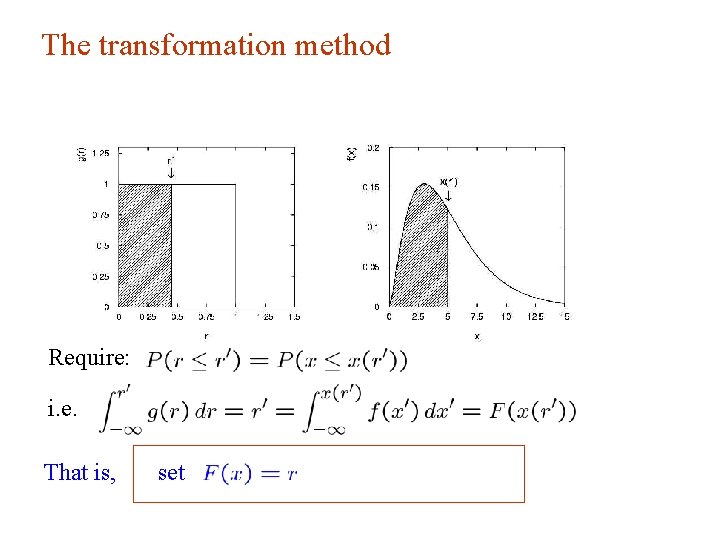
The transformation method Require: i. e. That is, set

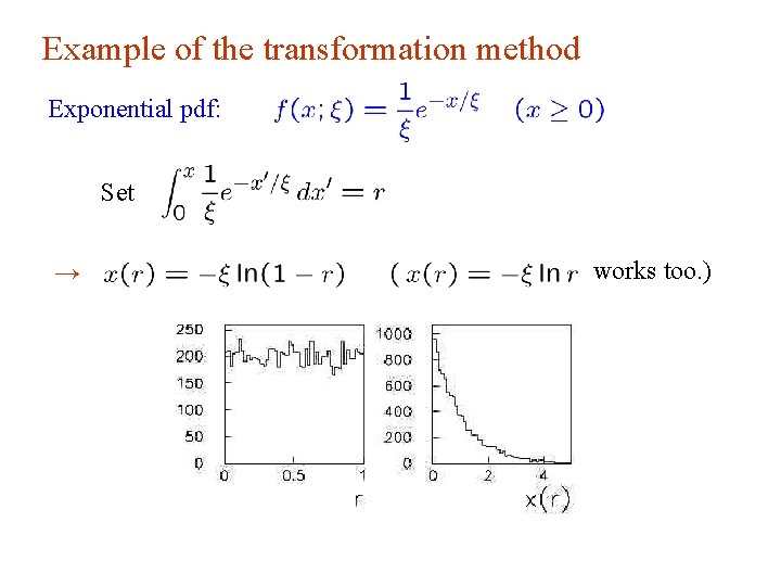
Example of the transformation method Exponential pdf: Set → works too. )

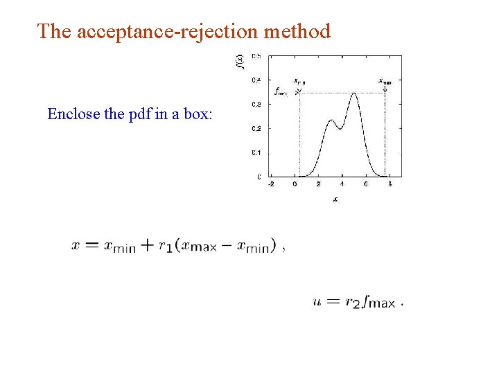
The acceptance-rejection method Enclose the pdf in a box:

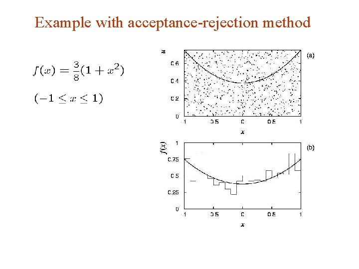
Example with acceptance-rejection method

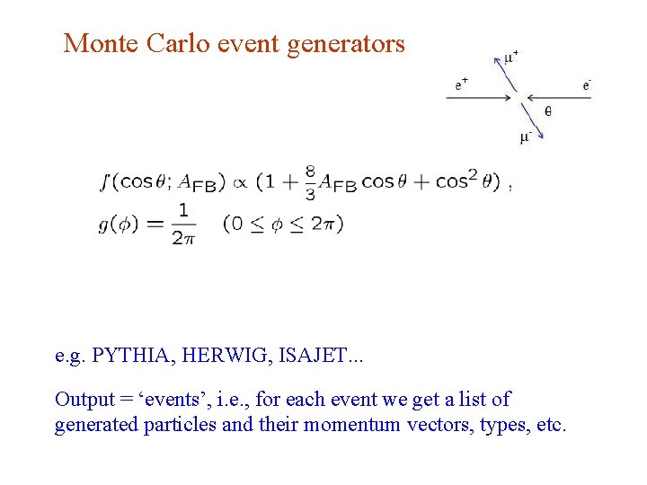
Monte Carlo event generators e. g. PYTHIA, HERWIG, ISAJET. . . Output = ‘events’, i. e. , for each event we get a list of generated particles and their momentum vectors, types, etc.

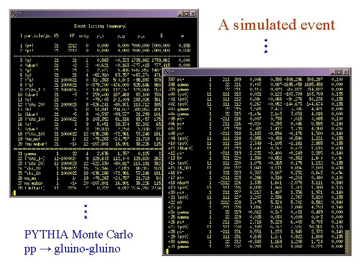
A simulated event PYTHIA Monte Carlo pp → gluino-gluino

Monte Carlo detector simulation

Wrapping up lecture 1 Up to now we’ve talked about properties of probability: definition and interpretation, Bayes’ theorem, random variables, probability (density) functions, expectation values (mean, variance, covariance. . . ) and we’ve looked at Monte Carlo, a numerical technique for computing quantities that can be related to probabilities. But suppose now we are faced with experimental data, and we want to infer something about the (probabilistic) processes that produced the data. This is statistics, the main subject of the following lectures.

Extra slides for lecture 1

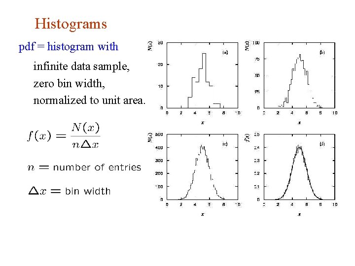
Histograms pdf = histogram with infinite data sample, zero bin width, normalized to unit area.

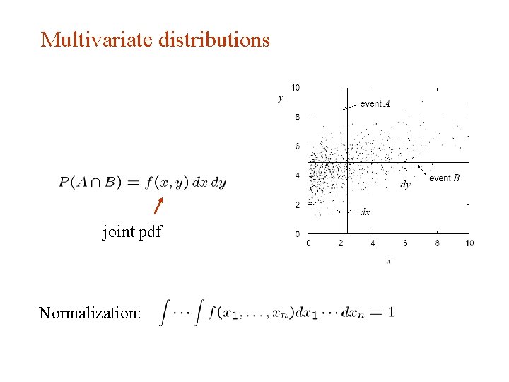
Multivariate distributions joint pdf Normalization:

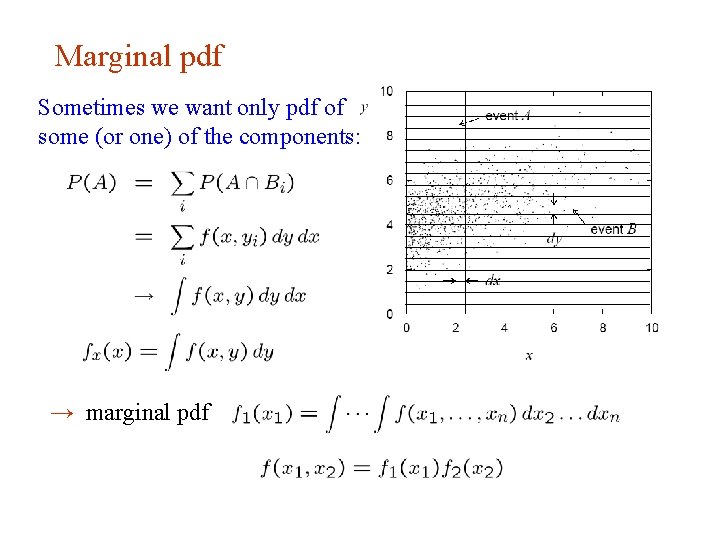
Marginal pdf Sometimes we want only pdf of some (or one) of the components: → marginal pdf

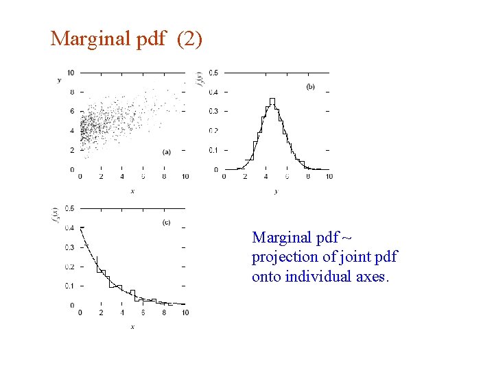
Marginal pdf (2) Marginal pdf ~ projection of joint pdf onto individual axes.

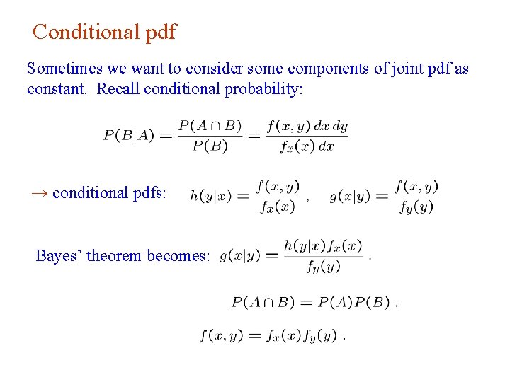
Conditional pdf Sometimes we want to consider some components of joint pdf as constant. Recall conditional probability: → conditional pdfs: Bayes’ theorem becomes:

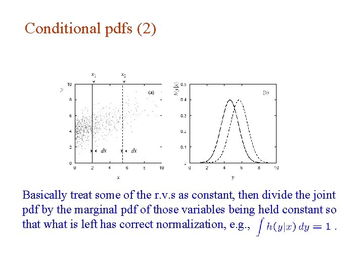
Conditional pdfs (2) Basically treat some of the r. v. s as constant, then divide the joint pdf by the marginal pdf of those variables being held constant so that what is left has correct normalization, e. g. ,

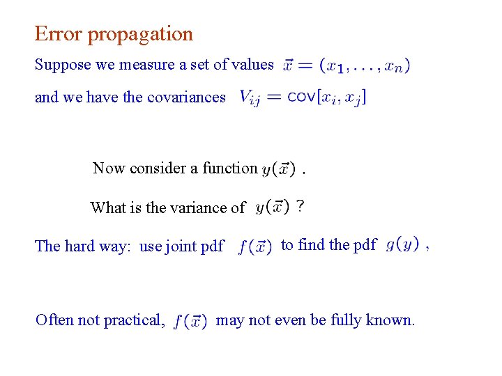
Error propagation Suppose we measure a set of values and we have the covariances Now consider a function What is the variance of The hard way: use joint pdf Often not practical, to find the pdf may not even be fully known.

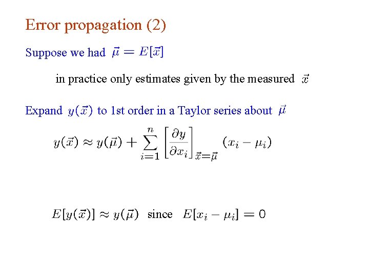
Error propagation (2) Suppose we had in practice only estimates given by the measured Expand to 1 st order in a Taylor series about since

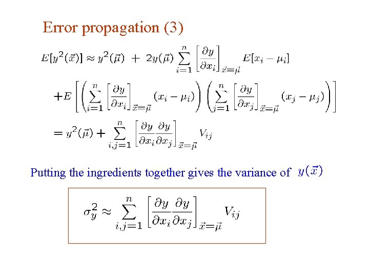
Error propagation (3) Putting the ingredients together gives the variance of

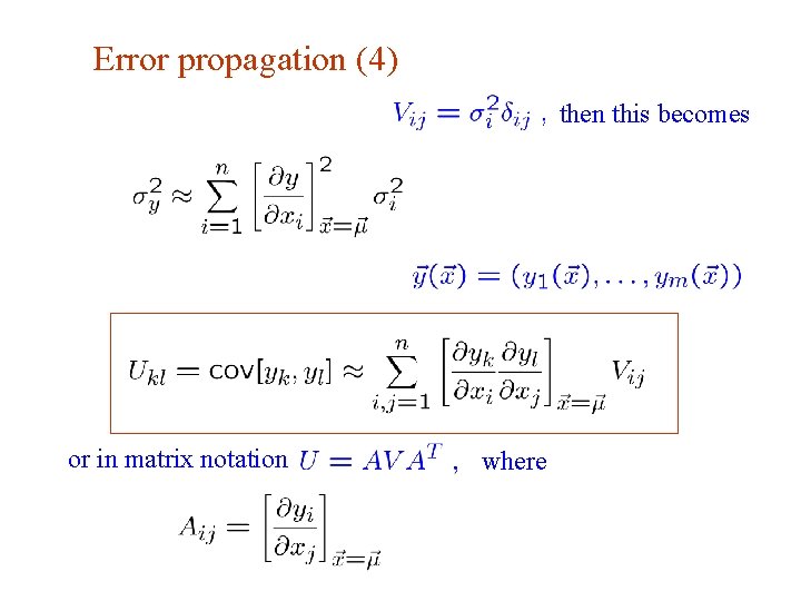
Error propagation (4) then this becomes or in matrix notation where

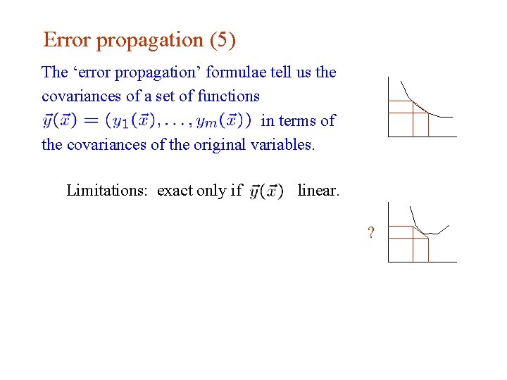
Error propagation (5) The ‘error propagation’ formulae tell us the covariances of a set of functions in terms of the covariances of the original variables. Limitations: exact only if linear. ?

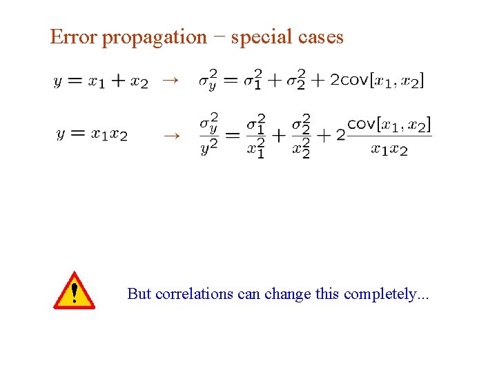
Error propagation − special cases → → But correlations can change this completely. . .

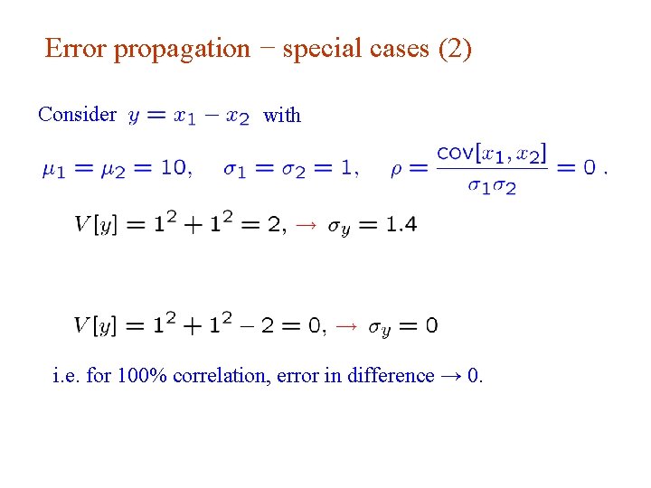
Error propagation − special cases (2) Consider with i. e. for 100% correlation, error in difference → 0.