Outline About Trondheim and myself Control structure design

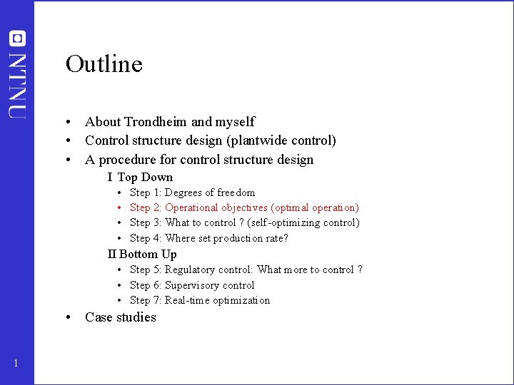
Outline • About Trondheim and myself • Control structure design (plantwide control) • A procedure for control structure design I Top Down • • Step 1: Degrees of freedom Step 2: Operational objectives (optimal operation) Step 3: What to control ? (self-optimizing control) Step 4: Where set production rate? II Bottom Up • Step 5: Regulatory control: What more to control ? • Step 6: Supervisory control • Step 7: Real-time optimization • Case studies 1

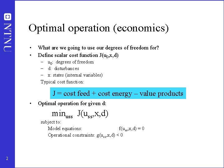
Optimal operation (economics) • • What are we going to use our degrees of freedom for? Define scalar cost function J(u 0, x, d) – u 0: degrees of freedom – d: disturbances – x: states (internal variables) Typical cost function: J = cost feed + cost energy – value products • Optimal operation for given d: minuss J(uss, x, d) subject to: Model equations: f(uss, x, d) = 0 Operational constraints: g(uss, x, d) < 0 2

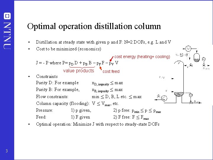
Optimal operation distillation column • • Distillation at steady state with given p and F: N=2 DOFs, e. g. L and V Cost to be minimized (economics) cost energy (heating+ cooling) J = - P where P= p. D D + p. B B – p. F F – p. V V value products 3 cost feed • Constraints Purity D: For example x. D, impurity · max Purity B: For example, x. B, impurity · max Flow constraints: min · D, B, L etc. · max Column capacity (flooding): V · Vmax, etc. Pressure: 1) p given, 2) p free: pmin · pmax Feed: 1) F given 2) F free: F · Fmax • Optimal operation: Minimize J with respect to steady-state DOFs

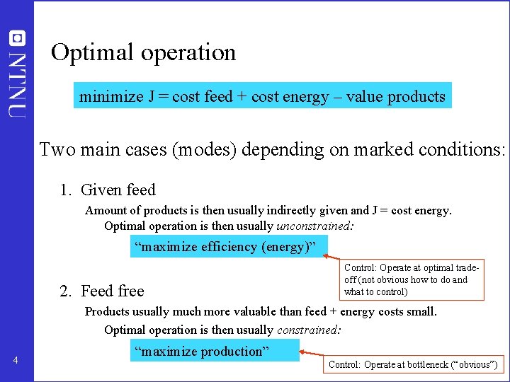
Optimal operation minimize J = cost feed + cost energy – value products Two main cases (modes) depending on marked conditions: 1. Given feed Amount of products is then usually indirectly given and J = cost energy. Optimal operation is then usually unconstrained: “maximize efficiency (energy)” 2. Feed free Control: Operate at optimal tradeoff (not obvious how to do and what to control) Products usually much more valuable than feed + energy costs small. Optimal operation is then usually constrained: 4 “maximize production” Control: Operate at bottleneck (“obvious”)

Comments optimal operation • Do not forget to include feedrate as a degree of freedom!! – For paper machine it may be optimal to have max. drying and adjust the speed of the paper machine! • Control at bottleneck – see later: “Where to set the production rate” 5

Outline • About Trondheim and myself • Control structure design (plantwide control) • A procedure for control structure design I Top Down • • Step 1: Degrees of freedom Step 2: Operational objectives (optimal operation) Step 3: What to control ? (self-optimizing control) Step 4: Where set production rate? II Bottom Up • Step 5: Regulatory control: What more to control ? • Step 6: Supervisory control • Step 7: Real-time optimization • Case studies 6

Step 3. What should we control (c)? (primary controlled variables y 1=c) Outline • Implementation of optimal operation • Self-optimizing control • Uncertainty (d and n) • Example: Marathon runner • Methods for finding the “magic” self-optimizing variables: A. Large gain: Minimum singular value rule B. “Brute force” loss evaluation C. Optimal combination of measurements • Example: Recycle process • Summary 7

Implementation of optimal operation • Optimal operation for given d*: minu J(u, x, d) subject to: Model equations: Operational constraints: → uopt(d*) f(u, x, d) = 0 g(u, x, d) < 0 Problem: Usally cannot keep uopt constant because disturbances d change How should be adjust the degrees of freedom (u)? 8

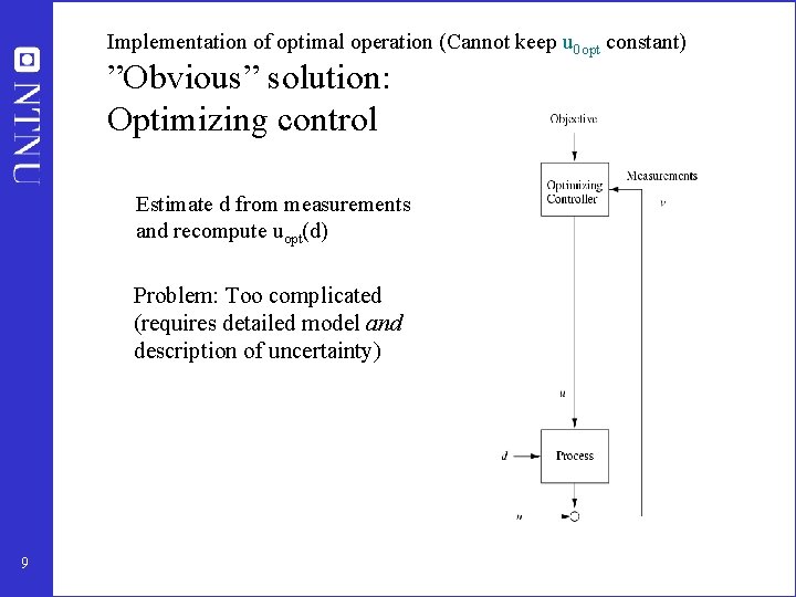
Implementation of optimal operation (Cannot keep u 0 opt constant) ”Obvious” solution: Optimizing control Estimate d from measurements and recompute uopt(d) Problem: Too complicated (requires detailed model and description of uncertainty) 9

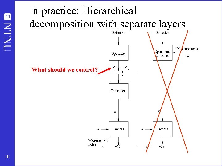
In practice: Hierarchical decomposition with separate layers What should we control? 10

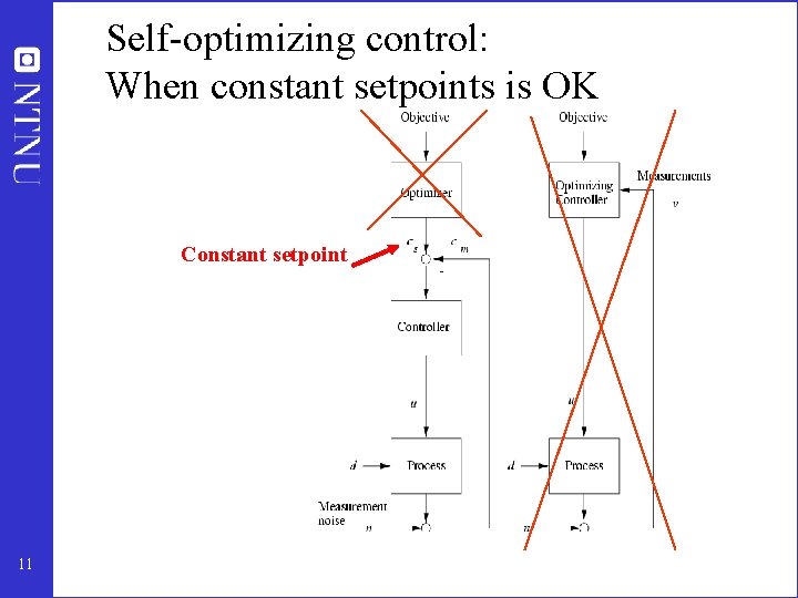
Self-optimizing control: When constant setpoints is OK Constant setpoint 11

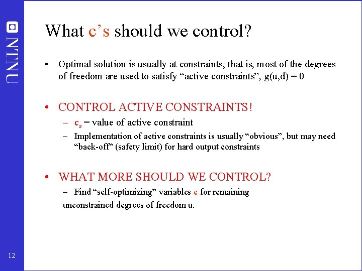
What c’s should we control? • Optimal solution is usually at constraints, that is, most of the degrees of freedom are used to satisfy “active constraints”, g(u, d) = 0 • CONTROL ACTIVE CONSTRAINTS! – cs = value of active constraint – Implementation of active constraints is usually “obvious”, but may need “back-off” (safety limit) for hard output constraints • WHAT MORE SHOULD WE CONTROL? – Find “self-optimizing” variables c for remaining unconstrained degrees of freedom u. 12

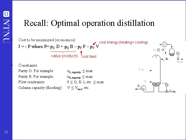
Recall: Optimal operation distillation • Cost to be minimized (economics) cost energy (heating+ cooling) J = - P where P= p. D D + p. B B – p. F F – p. V V value products cost feed • Constraints Purity D: For example Purity B: For example, Flow constraints: Column capacity (flooding): 13 x. D, impurity · max x. B, impurity · max 0 · D, B, L etc. · max V · Vmax, etc.

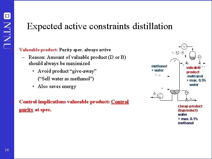
Expected active constraints distillation • Valueable product: Purity spec. always active – Reason: Amount of valuable product (D or B) should always be maximized • Avoid product “give-away” (“Sell water as methanol”) • Also saves energy • Control implications valueable product: Control purity at spec. 14 methanol + water valuable product methanol + max. 0. 5% water cheap product (byproduct) water + max. 0. 1% methanol

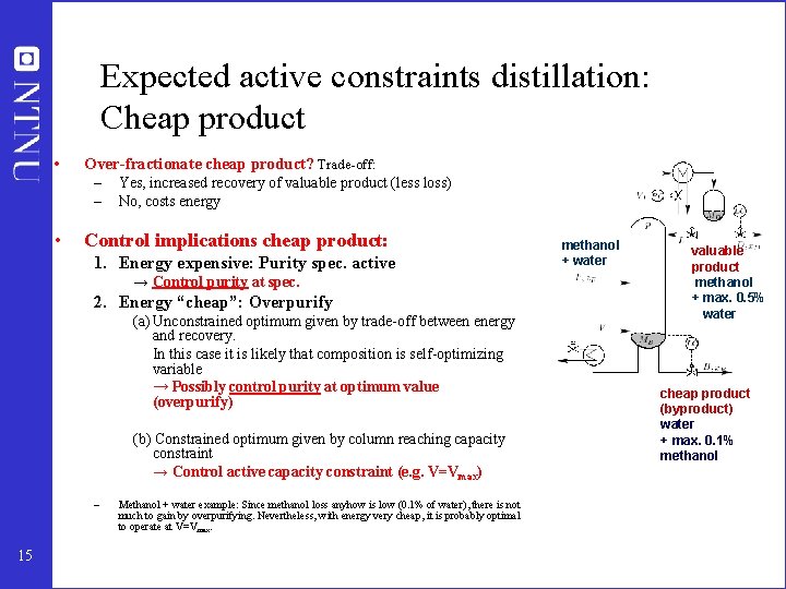
Expected active constraints distillation: Cheap product • Over-fractionate cheap product? Trade-off: – Yes, increased recovery of valuable product (less loss) – No, costs energy • Control implications cheap product: 1. Energy expensive: Purity spec. active → Control purity at spec. 2. Energy “cheap”: Overpurify (a) Unconstrained optimum given by trade-off between energy and recovery. In this case it is likely that composition is self-optimizing variable → Possibly control purity at optimum value (overpurify) (b) Constrained optimum given by column reaching capacity constraint → Control active capacity constraint (e. g. V=Vmax) – 15 Methanol + water example: Since methanol loss anyhow is low (0. 1% of water), there is not much to gain by overpurifying. Nevertheless, with energy very cheap, it is probably optimal to operate at V=Vmax. methanol + water valuable product methanol + max. 0. 5% water cheap product (byproduct) water + max. 0. 1% methanol

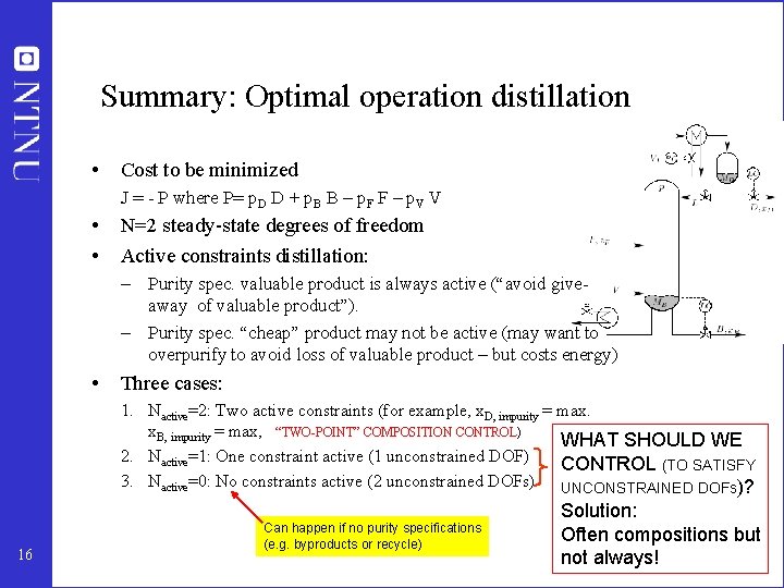
Summary: Optimal operation distillation • Cost to be minimized J = - P where P= p. D D + p. B B – p. F F – p. V V • • N=2 steady-state degrees of freedom Active constraints distillation: – Purity spec. valuable product is always active (“avoid giveaway of valuable product”). – Purity spec. “cheap” product may not be active (may want to overpurify to avoid loss of valuable product – but costs energy) • Three cases: 1. Nactive=2: Two active constraints (for example, x. D, impurity = max. x. B, impurity = max, “TWO-POINT” COMPOSITION CONTROL) WHAT SHOULD WE 2. Nactive=1: One constraint active (1 unconstrained DOF) CONTROL (TO SATISFY 3. Nactive=0: No constraints active (2 unconstrained DOFs) UNCONSTRAINED DOFs)? 16 Can happen if no purity specifications (e. g. byproducts or recycle) Solution: Often compositions but not always!

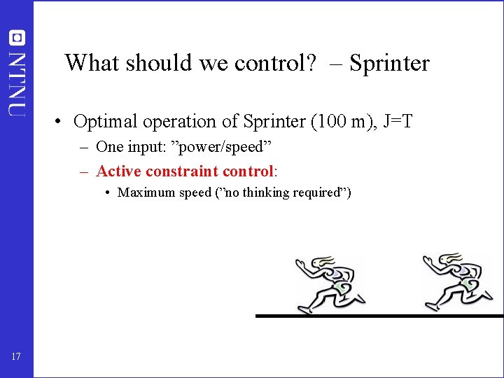
What should we control? – Sprinter • Optimal operation of Sprinter (100 m), J=T – One input: ”power/speed” – Active constraint control: • Maximum speed (”no thinking required”) 17

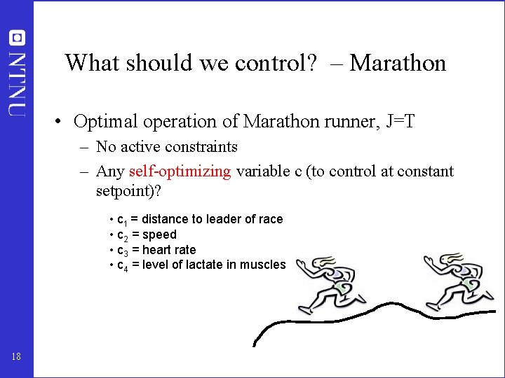
What should we control? – Marathon • Optimal operation of Marathon runner, J=T – No active constraints – Any self-optimizing variable c (to control at constant setpoint)? • c 1 = distance to leader of race • c 2 = speed • c 3 = heart rate • c 4 = level of lactate in muscles 18

Further examples self-optimizing control • • Marathon runner Central bank Cake baking Business systems (KPIs) Investment portifolio Biology Chemical process plants: Optimal blending of gasoline Define optimal operation (J) and look for ”magic” variable (c) which when kept constant gives acceptable loss (selfoptimizing control) 19

More on further examples • • • Central bank. J = welfare. u = interest rate. c=inflation rate (2. 5%) Cake baking. J = nice taste, u = heat input. c = Temperature (200 C) Business, J = profit. c = ”Key performance indicator (KPI), e. g. – Response time to order – Energy consumption pr. kg or unit – Number of employees – Research spending Optimal values obtained by ”benchmarking” • • Investment (portofolio management). J = profit. c = Fraction of investment in shares (50%) Biological systems: – ”Self-optimizing” controlled variables c have been found by natural selection – Need to do ”reverse engineering” : • • 20 Find the controlled variables used in nature From this possibly identify what overall objective J the biological system has been attempting to optimize

Unconstrained variables: What should we control? • Intuition: “Dominant variables” (Shinnar) • Is there any systematic procedure? 21

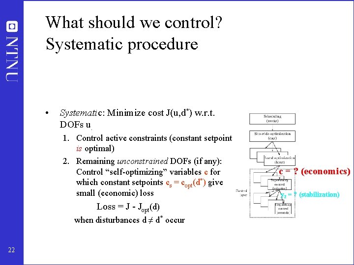
What should we control? Systematic procedure • Systematic: Minimize cost J(u, d*) w. r. t. DOFs u. 1. Control active constraints (constant setpoint is optimal) 2. Remaining unconstrained DOFs (if any): Control “self-optimizing” variables c for which constant setpoints cs = copt(d*) give small (economic) loss Loss = J - Jopt(d) when disturbances d ≠ d* occur 22 c = ? (economics) y 2 = ? (stabilization)

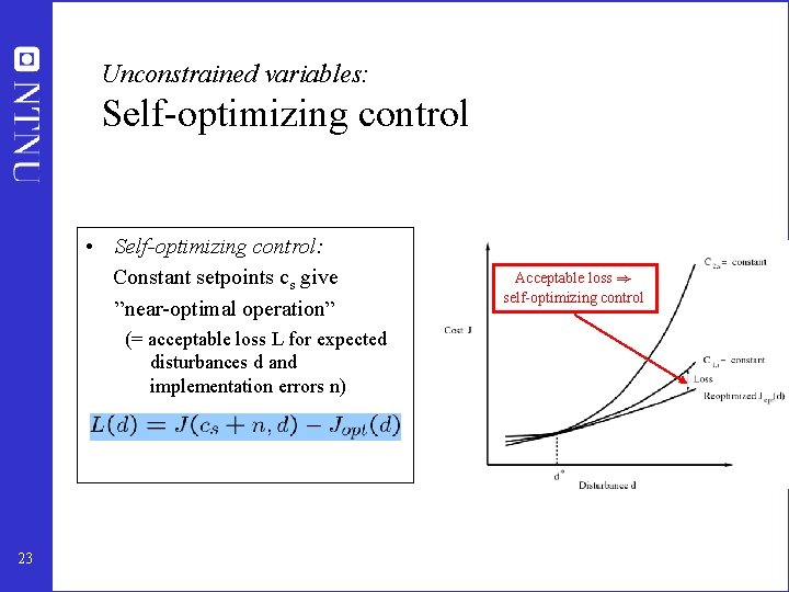
Unconstrained variables: Self-optimizing control • Self-optimizing control: Constant setpoints cs give ”near-optimal operation” (= acceptable loss L for expected disturbances d and implementation errors n) 23 Acceptable loss ) self-optimizing control

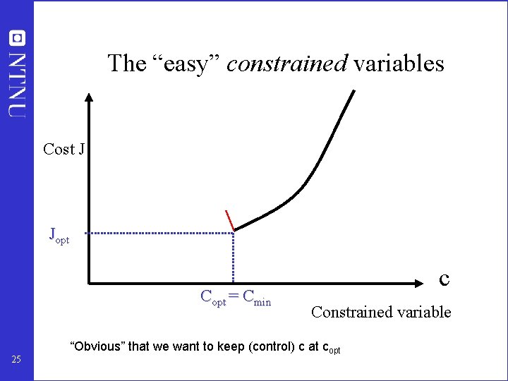
The “easy” constrained variables Cost J Jopt Copt = Cmin 25 c Constrained variable “Obvious” that we want to keep (control) c at copt

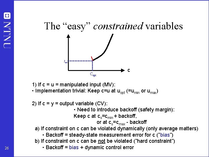
The “easy” constrained variables Jopt Copt c 1) If c = u = manipulated input (MV): • Implementation trivial: Keep c=u at uopt (=umin or umax) 26 2) If c = y = output variable (CV): • Need to introduce backoff (safety margin): Keep c at cs=cmin + backoff, or at cs=cmax - backoff a) If constraint on c can be violated dynamically (only average matters) • Backoff = steady-state measurement error for c (”bias”) b) If constraint on c can be not be violated (”hard constraint”) • Backoff = bias + dynamic control error

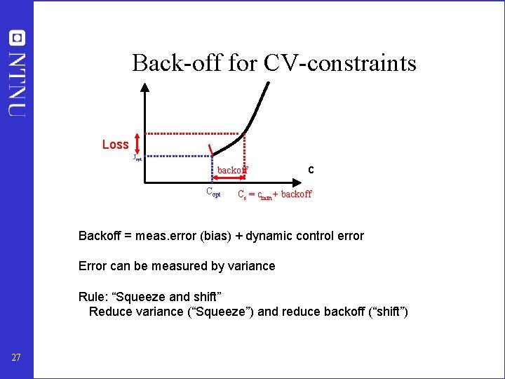
Back-off for CV-constraints Loss Jopt backoff Copt c Cs = cmin + backoff Backoff = meas. error (bias) + dynamic control error Error can be measured by variance Rule: “Squeeze and shift” Reduce variance (“Squeeze”) and reduce backoff (“shift”) 27

« SQUEEZE AND SHIFT » 28 © Richalet

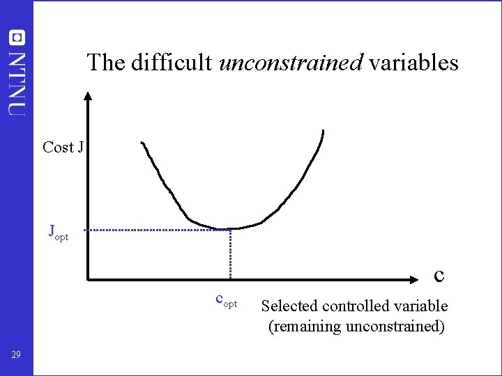
The difficult unconstrained variables Cost J Jopt c copt 29 Selected controlled variable (remaining unconstrained)

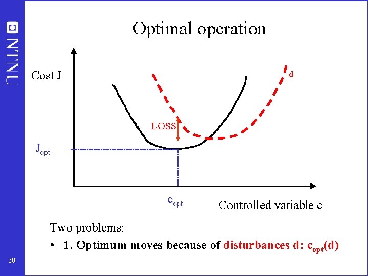
Optimal operation Cost J d LOSS Jopt copt Controlled variable c Two problems: • 1. Optimum moves because of disturbances d: copt(d) 30

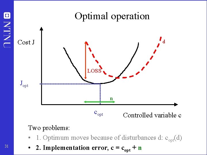
Optimal operation Cost J d LOSS Jopt n copt 31 Controlled variable c Two problems: • 1. Optimum moves because of disturbances d: copt(d) • 2. Implementation error, c = copt + n

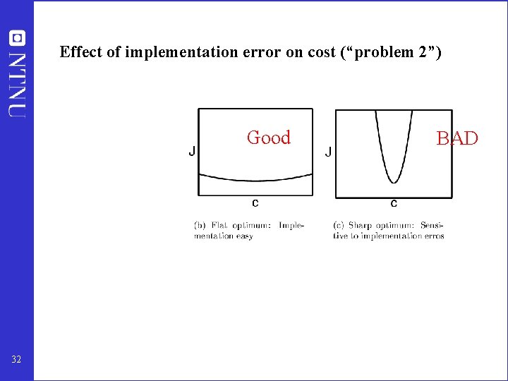
Effect of implementation error on cost (“problem 2”) Good 32 BAD

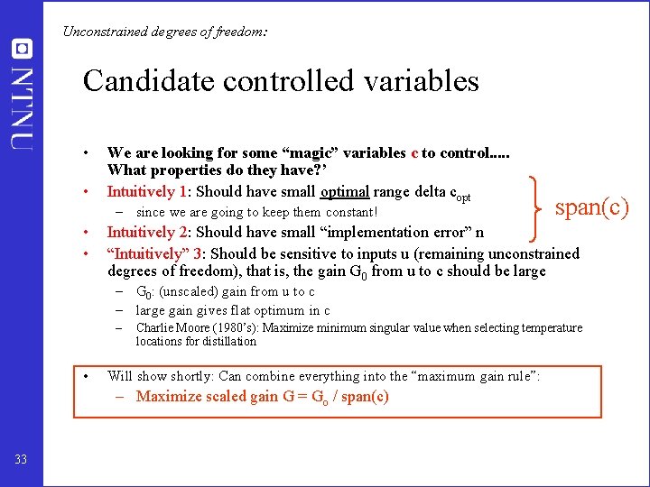
Unconstrained degrees of freedom: Candidate controlled variables • • We are looking for some “magic” variables c to control. . . What properties do they have? ’ Intuitively 1: Should have small optimal range delta copt – since we are going to keep them constant! • • span(c) Intuitively 2: Should have small “implementation error” n “Intuitively” 3: Should be sensitive to inputs u (remaining unconstrained degrees of freedom), that is, the gain G 0 from u to c should be large – G 0: (unscaled) gain from u to c – large gain gives flat optimum in c – • Charlie Moore (1980’s): Maximize minimum singular value when selecting temperature locations for distillation Will show shortly: Can combine everything into the “maximum gain rule”: – Maximize scaled gain G = Go / span(c) 33

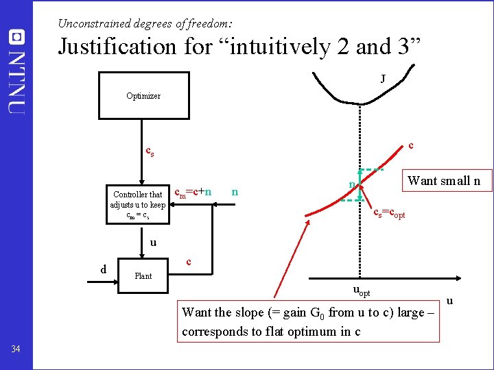
Unconstrained degrees of freedom: Justification for “intuitively 2 and 3” J Optimizer c cs Controller that adjusts u to keep cm = cs cm=c+n n Want small n n cs=copt u d c Plant uopt Want the slope (= gain G 0 from u to c) large – corresponds to flat optimum in c 34 u

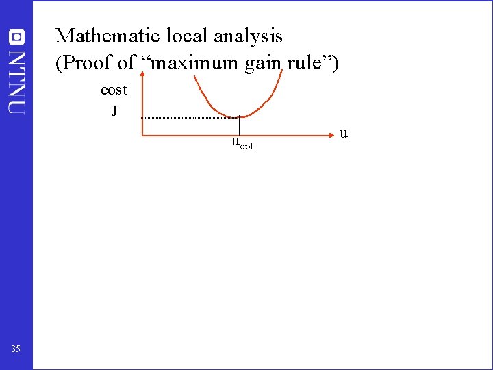
Mathematic local analysis (Proof of “maximum gain rule”) cost J uopt 35 u

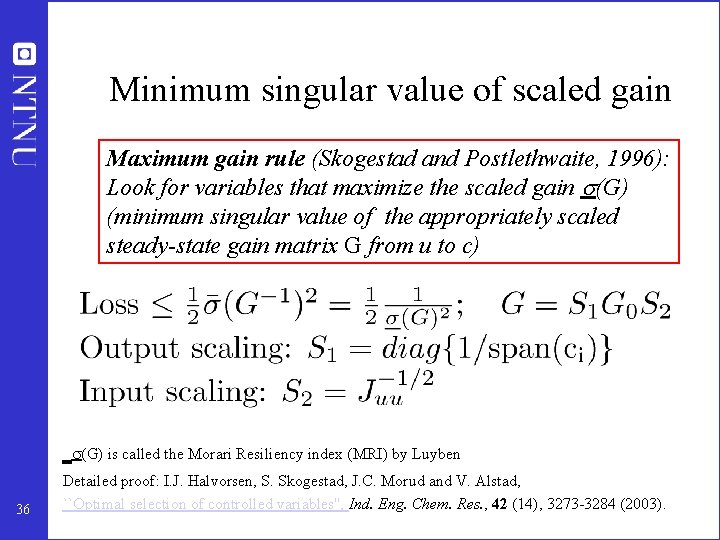
Minimum singular value of scaled gain Maximum gain rule (Skogestad and Postlethwaite, 1996): Look for variables that maximize the scaled gain (G) (minimum singular value of the appropriately scaled steady-state gain matrix G from u to c) (G) is called the Morari Resiliency index (MRI) by Luyben 36 Detailed proof: I. J. Halvorsen, S. Skogestad, J. C. Morud and V. Alstad, ``Optimal selection of controlled variables'', Ind. Eng. Chem. Res. , 42 (14), 3273 -3284 (2003).

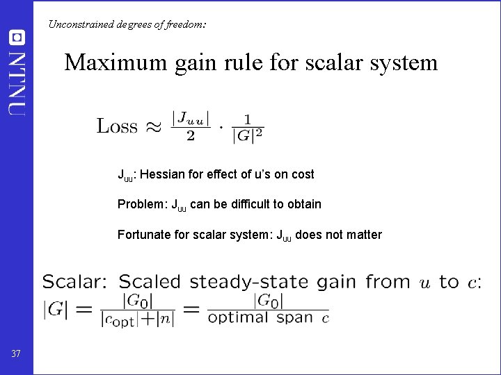
Unconstrained degrees of freedom: Maximum gain rule for scalar system Juu: Hessian for effect of u’s on cost Problem: Juu can be difficult to obtain Fortunate for scalar system: Juu does not matter 37

Maximum gain rule in words Select controlled variables c for which the gain G 0 (=“controllable range”) is large compared to its span (=sum of optimal variation and control error) 38

B. “Brute-force” procedure for selecting (primary) controlled variables (Skogestad, 2000) • • Step 1 Determine DOFs for optimization Step 2 Definition of optimal operation J (cost and constraints) Step 3 Identification of important disturbances Step 4 Optimization (nominally and with disturbances) Step 5 Identification of candidate controlled variables (use active constraint control) Step 6 Evaluation of loss with constant setpoints for alternative controlled variables : Check in particular for feasibility Step 7 Evaluation and selection (including controllability analysis) Case studies: Tenneessee-Eastman, Propane-propylene splitter, recycle process, heat-integrated distillation 39

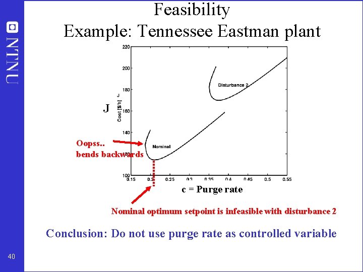
Feasibility Example: Tennessee Eastman plant J Oopss. . bends backwards c = Purge rate Nominal optimum setpoint is infeasible with disturbance 2 Conclusion: Do not use purge rate as controlled variable 40

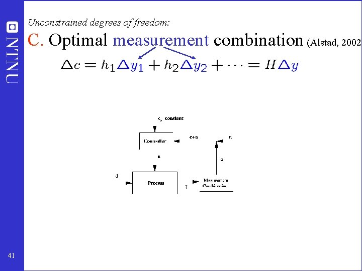
Unconstrained degrees of freedom: C. Optimal measurement combination (Alstad, 2002) 41

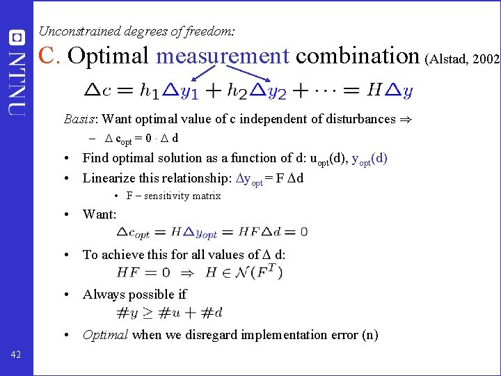
Unconstrained degrees of freedom: C. Optimal measurement combination (Alstad, 2002) Basis: Want optimal value of c independent of disturbances ) – copt = 0 ¢ d • Find optimal solution as a function of d: uopt(d), yopt(d) • Linearize this relationship: yopt = F d • F – sensitivity matrix • Want: • To achieve this for all values of d: • Always possible if • Optimal when we disregard implementation error (n) 42

Alstad-method continued • To handle implementation error: Use “sensitive” measurements, with information about all independent variables (u and d) 43

Summary unconstrained degrees of freedom: Looking for “magic” variables to keep at constant setpoints. How can we find them systematically? Candidates A. Start with: Maximum gain (minimum singular value) rule: B. Then: “Brute force evaluation” of most promising alternatives. Evaluate loss when the candidate variables c are kept constant. In particular, may be problem with feasibility C. If no good single candidates: Consider linear combinations (matrix H): 44

Toy Example 45

Toy Example 46

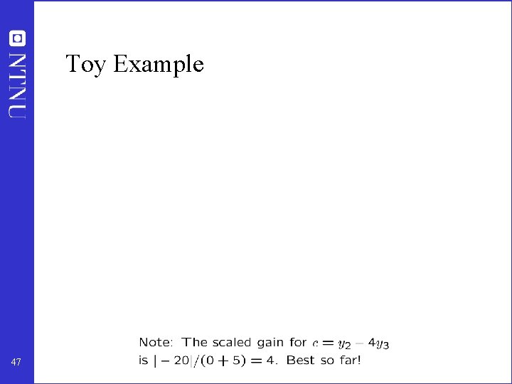
Toy Example 47

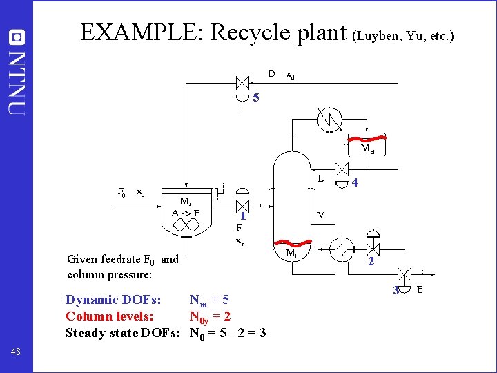
EXAMPLE: Recycle plant (Luyben, Yu, etc. ) 5 4 1 Given feedrate F 0 and column pressure: Dynamic DOFs: Nm = 5 Column levels: N 0 y = 2 Steady-state DOFs: N 0 = 5 - 2 = 3 48 2 3

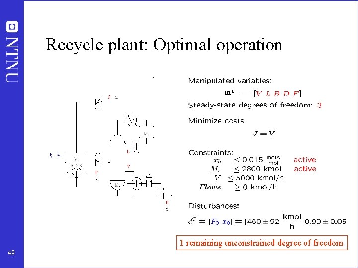
Recycle plant: Optimal operation m. T 1 remaining unconstrained degree of freedom 49

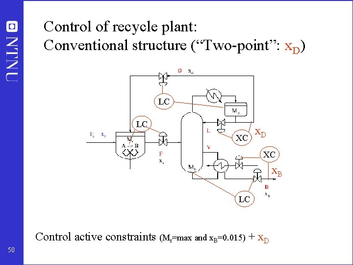
Control of recycle plant: Conventional structure (“Two-point”: x. D) LC LC XC x. D XC x. B LC Control active constraints (Mr=max and x. B=0. 015) + x. D 50

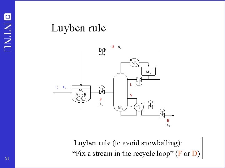
Luyben rule 51 Luyben rule (to avoid snowballing): “Fix a stream in the recycle loop” (F or D)

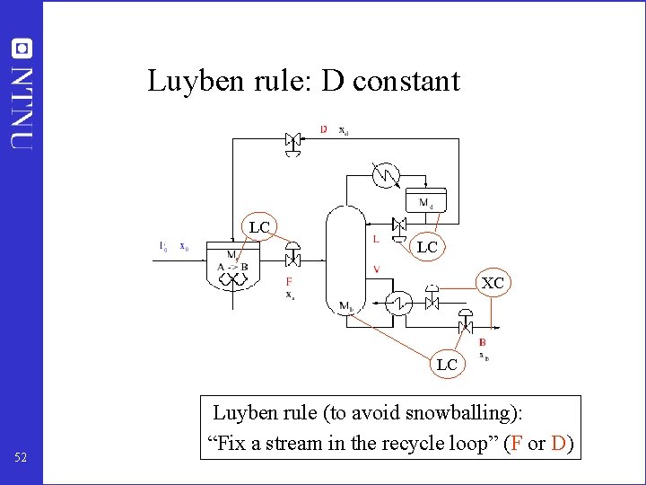
Luyben rule: D constant LC LC XC LC 52 Luyben rule (to avoid snowballing): “Fix a stream in the recycle loop” (F or D)

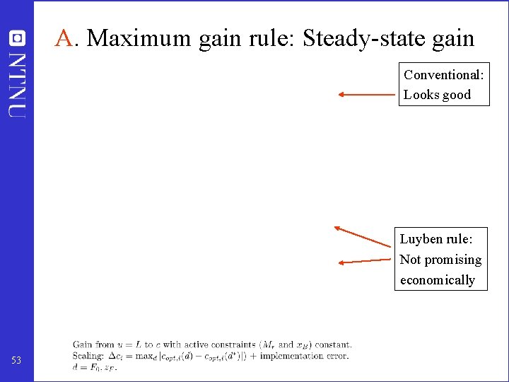
A. Maximum gain rule: Steady-state gain Conventional: Looks good Luyben rule: Not promising economically 53

How did we find the gains in the Table? 1. Find nominal optimum 2. Find (unscaled) gain G 0 from input to candidate outputs: c = G 0 u. • • In this case only a single unconstrained input (DOF). Choose at u=L Obtain gain G 0 numerically by making a small perturbation in u=L while adjusting the other inputs such that the active constraints are constant (bottom composition fixed in this case) IMPORTANT! 3. Find the span for each candidate variable • • • For each disturbance di make a typical change and reoptimize to obtain the optimal ranges copt(di) For each candidate output obtain (estimate) the control error (noise) n The expected variation for c is then: span(c) = i | copt(di)| + |n| 4. Obtain the scaled gain, G = |G 0| / span(c) 5. 54 Note: The absolute value (the vector 1 -norm) is used here to "sum up" and get the overall span. Alternatively, the 2 -norm could be used, which could be viewed as putting less emphasis on the worst case. As an example, assume that the only contribution to the span is the implementation/measurement error, and that the variable we are controlling (c) is the average of 5 measurements of the same y, i. e. c=sum yi/5, and that each yi has a measurement error of 1, i. e. nyi=1. Then with the absolute value (1 -norm), the contribution to the span from the implementation (meas. ) error is span=sum abs(nyi)/5 = 5*1/5=1, whereas with the two-norn, span = sqrt(5*(1/5^2) = 0. 447. The latter is more reasonable since we expect that the overall measurement error is reduced when taking the average of many measurements. In any case, the choice of norm is an engineering decision so there is not really one that is "right" and one that is "wrong". We often use the 2 -norm for mathematical convenience, but there also physical justifications (as just given!).

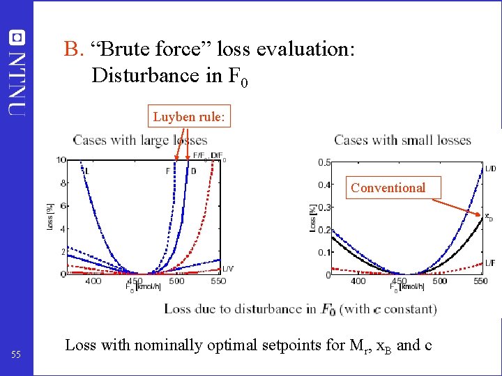
B. “Brute force” loss evaluation: Disturbance in F 0 Luyben rule: Conventional 55 Loss with nominally optimal setpoints for Mr, x. B and c

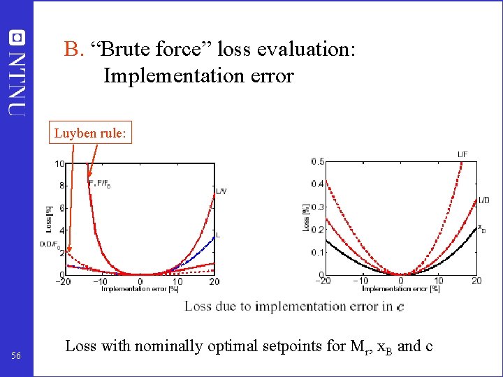
B. “Brute force” loss evaluation: Implementation error Luyben rule: 56 Loss with nominally optimal setpoints for Mr, x. B and c

C. Optimal measurement combination • 1 unconstrained variable (#c = 1) • 1 (important) disturbance: F 0 (#d = 1) • “Optimal” combination requires 2 “measurements” (#y = #u + #d = 2) – For example, c = h 1 L + h 2 F • BUT: Not much to be gained compared to control of single variable (e. g. L/F or x. D) 57

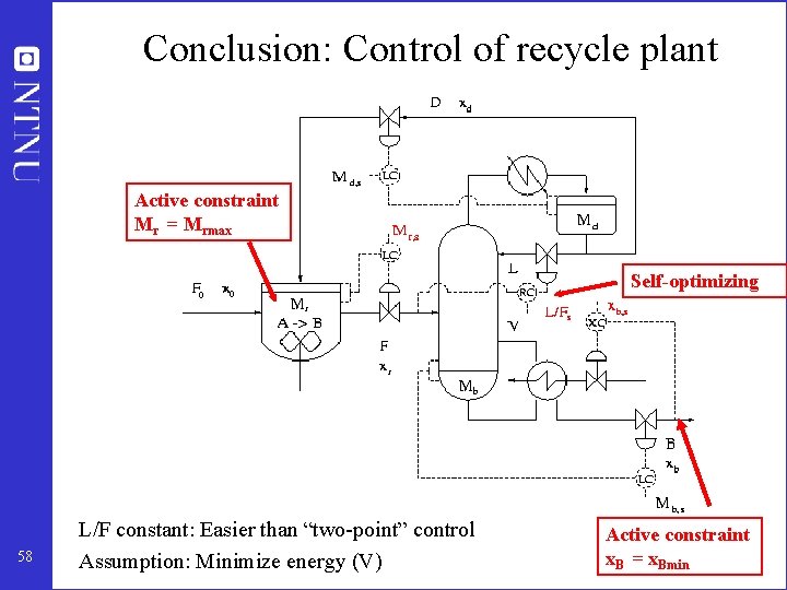
Conclusion: Control of recycle plant Active constraint Mr = Mrmax Self-optimizing 58 L/F constant: Easier than “two-point” control Assumption: Minimize energy (V) Active constraint x. B = x. Bmin

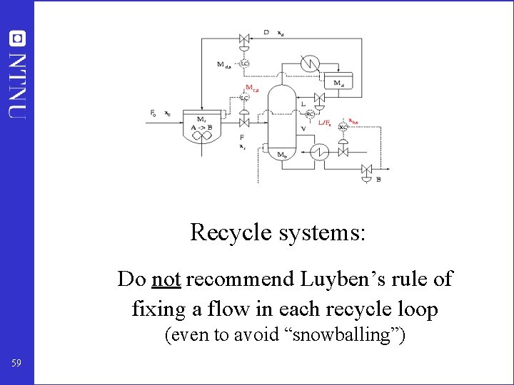
Recycle systems: Do not recommend Luyben’s rule of fixing a flow in each recycle loop (even to avoid “snowballing”) 59

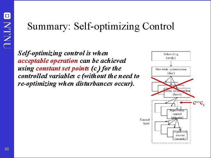
Summary: Self-optimizing Control Self-optimizing control is when acceptable operation can be achieved using constant set points (cs) for the controlled variables c (without the need to re-optimizing when disturbances occur). c=cs 60

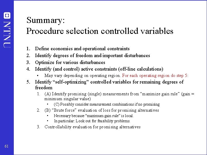
Summary: Procedure selection controlled variables 1. 2. 3. 4. Define economics and operational constraints Identify degrees of freedom and important disturbances Optimize for various disturbances Identify (and control) active constraints (off-line calculations) • May vary depending on operating region. For each operating region do step 5: 5. Identify “self-optimizing” controlled variables for remaining degrees of freedom 1. (A) Identify promising (single) measurements from “maximize gain rule” (gain = minimum singular value) • (C) Possibly consider measurement combinations if no promising 2. (B) “Brute force” evaluation of loss for promising alternatives • • Necessary because “maximum gain rule” is local. In particular: Look out for feasibility problems. 3. Controllability evaluation for promising alternatives 61

Summary ”self-optimizing” control • Operation of most real system: Constant setpoint policy (c = cs) – – • Central bank Business systems: KPI’s Biological systems Chemical processes Goal: Find controlled variables c such that constant setpoint policy gives acceptable operation in spite of uncertainty ) Self-optimizing control • • • Method A: Maximize (G) Method B: Evaluate loss L = J - Jopt Method C: Optimal linear measurement combination: c = H y where HF=0 62

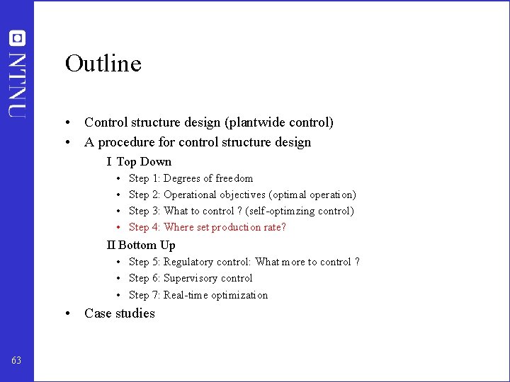
Outline • Control structure design (plantwide control) • A procedure for control structure design I Top Down • • Step 1: Degrees of freedom Step 2: Operational objectives (optimal operation) Step 3: What to control ? (self-optimzing control) Step 4: Where set production rate? II Bottom Up • Step 5: Regulatory control: What more to control ? • Step 6: Supervisory control • Step 7: Real-time optimization • Case studies 63