Our Recent Research Efforts AXing Zhu and James

Our Recent Research Efforts A-Xing Zhu and James E. Burt Department of Geography, University of Wisconsin-Madison, Wisconsin, USA

Outline 1. Neighborhood Size Effects 2. Purposive Sampling

Impact of Neighborhood Size on Terrain Derivatives and Digital Soil Mapping A-Xing Zhu, James E. Burt, Michael Smith, Rongxun Wang, Jing Gao Department of Geography, University of Wisconsin-Madison, Wisconsin, USA

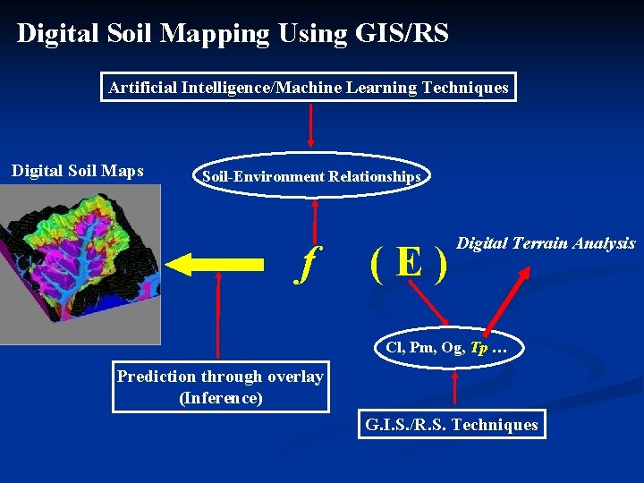
Digital Soil Mapping Using GIS/RS Artificial Intelligence/Machine Learning Techniques Digital Soil Maps Soil-Environment Relationships f (E) Digital Terrain Analysis Cl, Pm, Og, Tp … Prediction through overlay (Inference) G. I. S. /R. S. Techniques

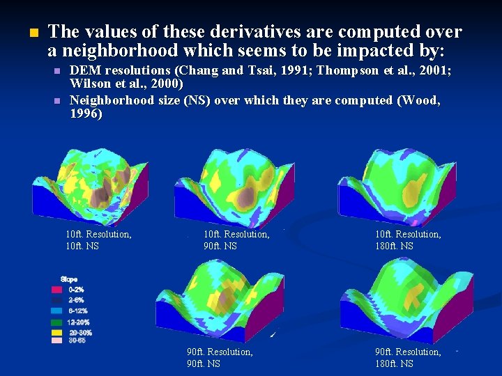
n The values of these derivatives are computed over a neighborhood which seems to be impacted by: n n DEM resolutions (Chang and Tsai, 1991; Thompson et al. , 2001; Wilson et al. , 2000) Neighborhood size (NS) over which they are computed (Wood, 1996) 10 ft. Resolution, 10 ft. NS 10 ft. Resolution, 90 ft. NS 90 ft. Resolution, 90 ft. NS 10 ft. Resolution, 180 ft. NS 90 ft. Resolution, 180 ft. NS

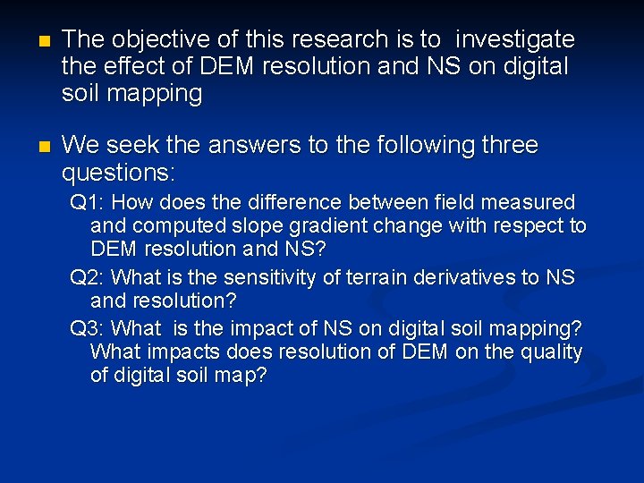
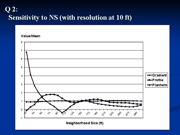
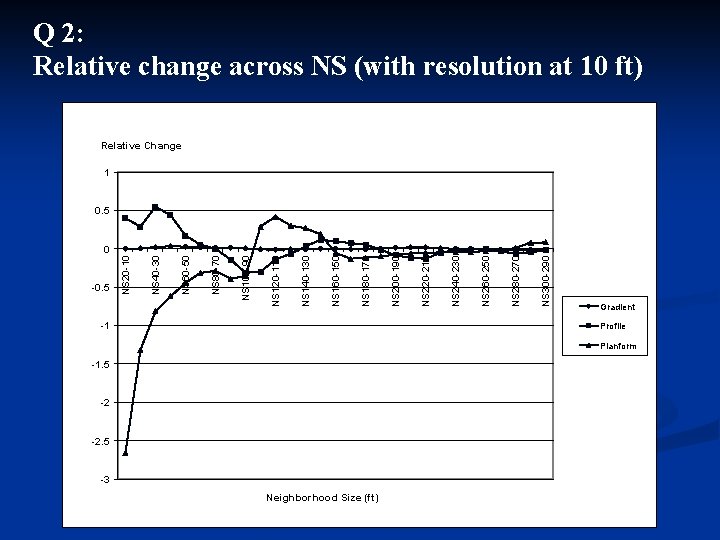
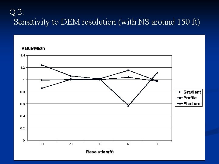
n The objective of this research is to investigate the effect of DEM resolution and NS on digital soil mapping n We seek the answers to the following three questions: Q 1: How does the difference between field measured and computed slope gradient change with respect to DEM resolution and NS? Q 2: What is the sensitivity of terrain derivatives to NS and resolution? Q 3: What is the impact of NS on digital soil mapping? What impacts does resolution of DEM on the quality of digital soil map?

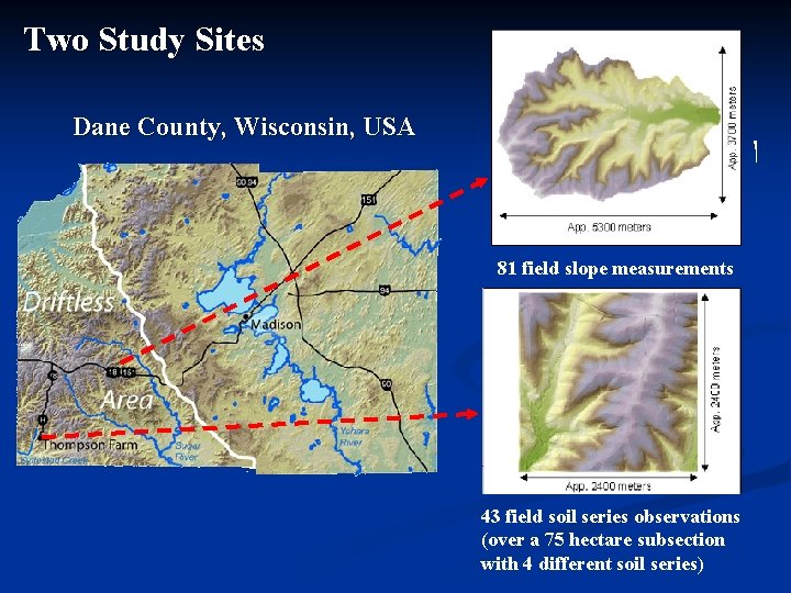
Two Study Sites Dane County, Wisconsin, USA 81 field slope measurements 43 field soil series observations (over a 75 hectare subsection with 4 different soil series)

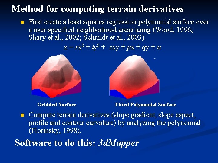
Method for computing terrain derivatives n First create a least squares regression polynomial surface over a user-specified neighborhood areas using (Wood, 1996; Shary et al. , 2002; Schmidt et al. , 2003): z = rx 2 + ty 2 + sxy + px + qy + u Gridded Surface n Fitted Polynomial Surface Compute terrain derivatives (slope gradient, slope aspect, profile and contour curvature) by analyzing the polynomial (Florinsky, 1998). Software to do this: 3 d. Mapper

Experiment Design n Original Elevation data sources: n n n a 10 ft. DEM from a 2000 air photography a 30 ft. DEM from a 1995 air photography Coarsening the 10 ft. DEM to 15 ft. , 20 ft. , 25 ft. , 30 ft. , 35 ft. 40 ft. , 45 ft. , 50 ft EMs using the nearest neighbor approach in ESRI Arc/INFO. Coarsening the 30 ft. DEM to 35 ft. 40 ft. , 45 ft. , 50 ft. DEMs using the nearest neighbor approach in ESRI Arc/INFO. Values of terrain derivatives were computed for each DEM resolution over each neighborhood size, up to 300 ft. with 5 ft increment

Q 1: Difference in slope gradient by NS and resolution Observations: 1. The difference is smallest not at the finest neighborhood size, but rather at some larger size, about 100 feet in this case 2. Resolution does not seem to play a role

Q 2: Sensitivity to NS (with resolution at 10 ft) Value/Mean 8 7 6 5 Gradient Profile Planform 4 3 2 1 -1 Neighborhood Size (ft) 29 0 27 0 25 0 23 0 21 0 19 0 17 0 15 0 13 0 11 0 90 70 50 30 10 0

Q 2: Relative change across NS (with resolution at 10 ft) Relative Change 1 0. 5 -1 NS 300 -290 NS 280 -270 NS 260 -250 NS 240 -230 NS 220 -210 NS 200 -190 NS 180 -170 NS 160 -150 NS 140 -130 NS 120 -110 NS 100 -90 NS 80 -70 NS 60 -50 NS 40 -30 -0. 5 NS 20 -10 0 Gradient Profile Planform -1. 5 -2 -2. 5 -3 Neighborhood Size (ft)

Q 2: Sensitivity to DEM resolution (with NS around 150 ft) Value/Mean 1. 4 1. 2 1 Gradient Profile Planform 0. 8 0. 6 0. 4 0. 2 0 10 20 30 Resolution(ft) 40 50

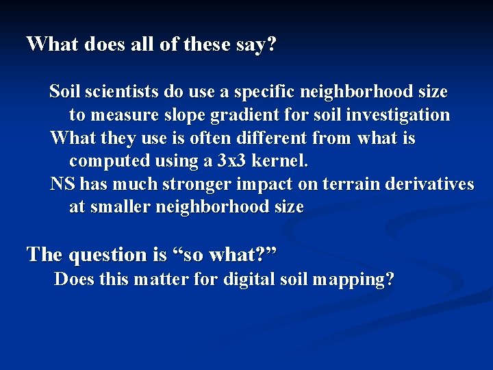
What does all of these say? Soil scientists do use a specific neighborhood size to measure slope gradient for soil investigation What they use is often different from what is computed using a 3 x 3 kernel. NS has much stronger impact on terrain derivatives at smaller neighborhood size The question is “so what? ” Does this matter for digital soil mapping?

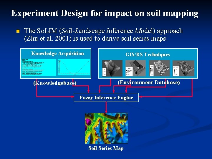
Experiment Design for impact on soil mapping n The So. LIM (Soil-Landscape Inference Model) approach (Zhu et al. 2001) is used to derive soil series maps: Knowledge Acquisition (Knowledgebase) GIS/RS Techniques (Environment Database) Fuzzy Inference Engine Soil Series Map

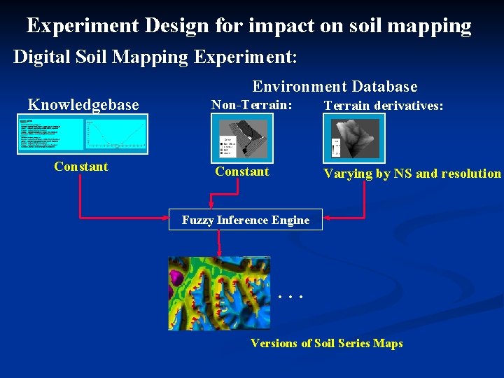
Experiment Design for impact on soil mapping Digital Soil Mapping Experiment: Knowledgebase Constant Environment Database Non-Terrain: Terrain derivatives: Constant Varying by NS and resolution Fuzzy Inference Engine … Versions of Soil Series Maps

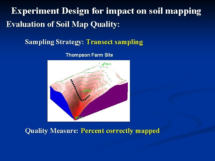
Experiment Design for impact on soil mapping Evaluation of Soil Map Quality: Sampling Strategy: Transect sampling Thompson Farm Site Quality Measure: Percent correctly mapped

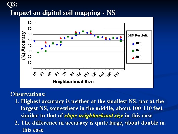
Q 3: Impact on digital soil mapping - NS 80 (%) Accuracy 70 60 DEM Resolution 50 10 ft. 40 30 15 ft. 20 30 ft. 10 17 0 16 0 14 0 13 0 11 0 10 0 80 70 50 40 20 10 0 Neighborhood Size Observations: 1. Highest accuracy is neither at the smallest NS, nor at the largest NS, somewhere in the middle, about 100 -110 feet similar to that of slope neighborhood size in this case 2. The difference in accuracy is quite large, about double in this case

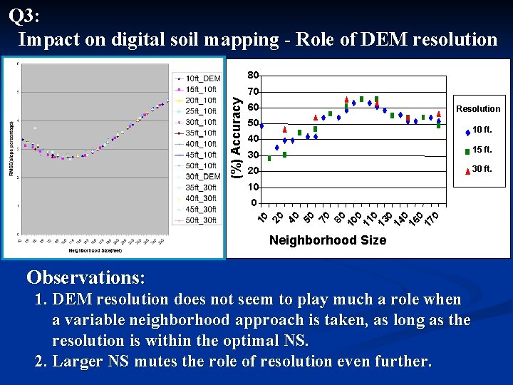
Q 3: Impact on digital soil mapping - Role of DEM resolution 80 (%) Accuracy 70 60 Resolution 50 10 ft. 40 15 ft. 30 30 ft. 20 10 70 80 10 0 11 0 13 0 14 0 16 0 17 0 40 50 10 20 0 Neighborhood Size Observations: 1. DEM resolution does not seem to play much a role when a variable neighborhood approach is taken, as long as the resolution is within the optimal NS. 2. Larger NS mutes the role of resolution even further.

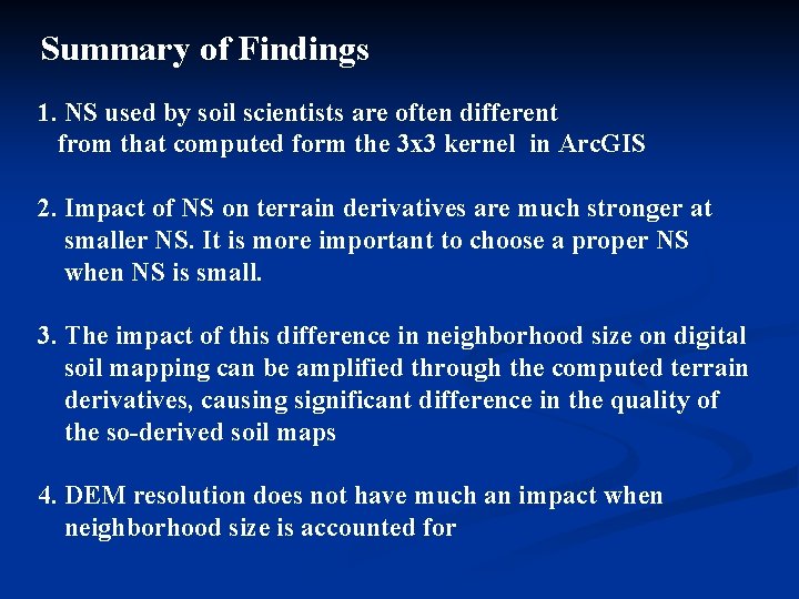
Summary of Findings 1. NS used by soil scientists are often different from that computed form the 3 x 3 kernel in Arc. GIS 2. Impact of NS on terrain derivatives are much stronger at smaller NS. It is more important to choose a proper NS when NS is small. 3. The impact of this difference in neighborhood size on digital soil mapping can be amplified through the computed terrain derivatives, causing significant difference in the quality of the so-derived soil maps 4. DEM resolution does not have much an impact when neighborhood size is accounted for

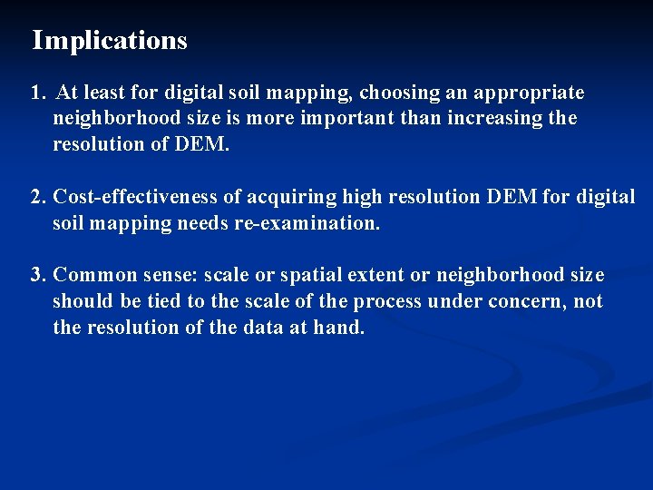
Implications 1. At least for digital soil mapping, choosing an appropriate neighborhood size is more important than increasing the resolution of DEM. 2. Cost-effectiveness of acquiring high resolution DEM for digital soil mapping needs re-examination. 3. Common sense: scale or spatial extent or neighborhood size should be tied to the scale of the process under concern, not the resolution of the data at hand.

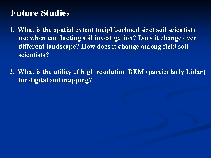
Future Studies 1. What is the spatial extent (neighborhood size) soil scientists use when conducting soil investigation? Does it change over different landscape? How does it change among field soil scientists? 2. What is the utility of high resolution DEM (particularly Lidar) for digital soil mapping?

Purposive Sampling for Digital Soil Mapping A-Xing Zhu 1, Baolin Li 2, Edward English 1 Lin Yang 2, Chengzhi Qin 2, James E. Burt 1, Chenghu Zhou 2 1 Department of Geography University of Wisconsin-Madison, USA 2 State Key Lab of Resources and Environmental Information System Institute of Geographical Sciences and Natural Resources Research Chinese Academy of Sciences, China

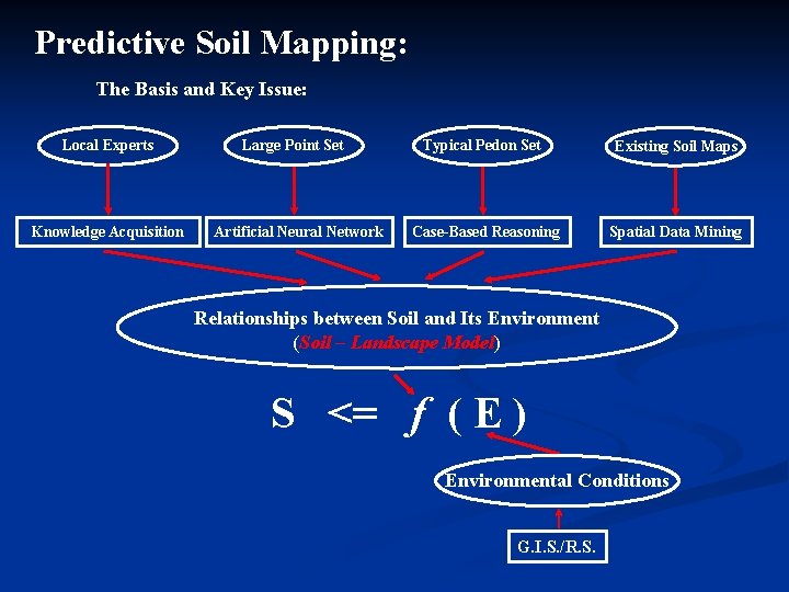
Predictive Soil Mapping: The Basis and Key Issue: Local Experts Knowledge Acquisition Large Point Set Artificial Neural Network Typical Pedon Set Existing Soil Maps Case-Based Reasoning Spatial Data Mining Relationships between Soil and Its Environment (Soil – Landscape Model) S <= f ( E ) Environmental Conditions G. I. S. /R. S.

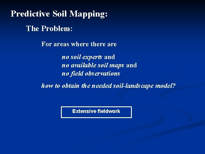
Predictive Soil Mapping: The Problem: For areas where there are no soil experts and no available soil maps and no field observations how to obtain the needed soil-landscape model? Extensive fieldwork

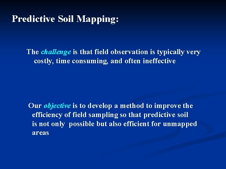
Predictive Soil Mapping: The challenge is that field observation is typically very costly, time consuming, and often ineffective Our objective is to develop a method to improve the efficiency of field sampling so that predictive soil is not only possible but also efficient for unmapped areas

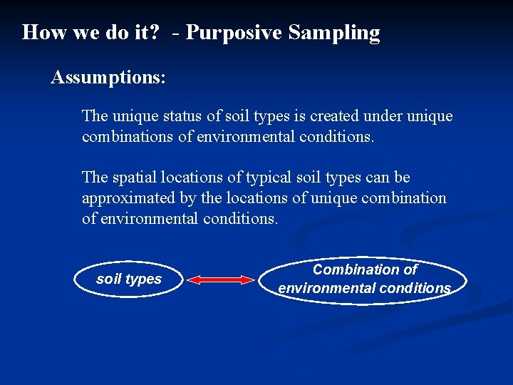
How we do it? - Purposive Sampling Assumptions: The unique status of soil types is created under unique combinations of environmental conditions. The spatial locations of typical soil types can be approximated by the locations of unique combination of environmental conditions. soil types Combination of environmental conditions

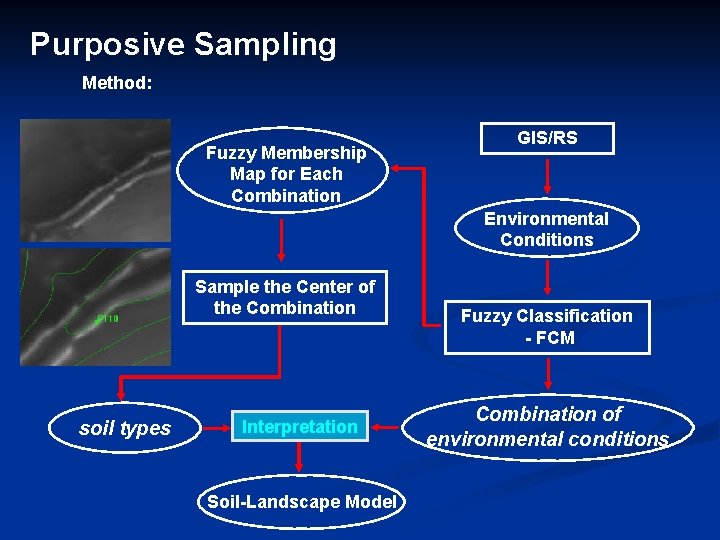
Purposive Sampling Method: Fuzzy Membership Map for Each Combination GIS/RS Environmental Conditions Sample the Center of the Combination soil types Interpretation Soil-Landscape Model Fuzzy Classification - FCM Combination of environmental conditions

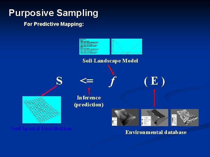
Purposive Sampling For Predictive Mapping: Soil-Landscape Model S <= f (E) Inference (prediction) Soil Spatial Distribution Environmental database

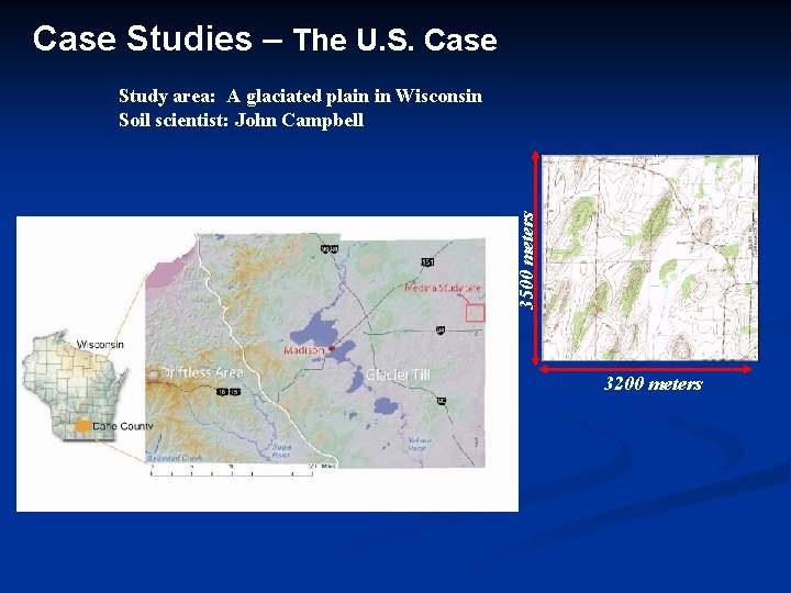
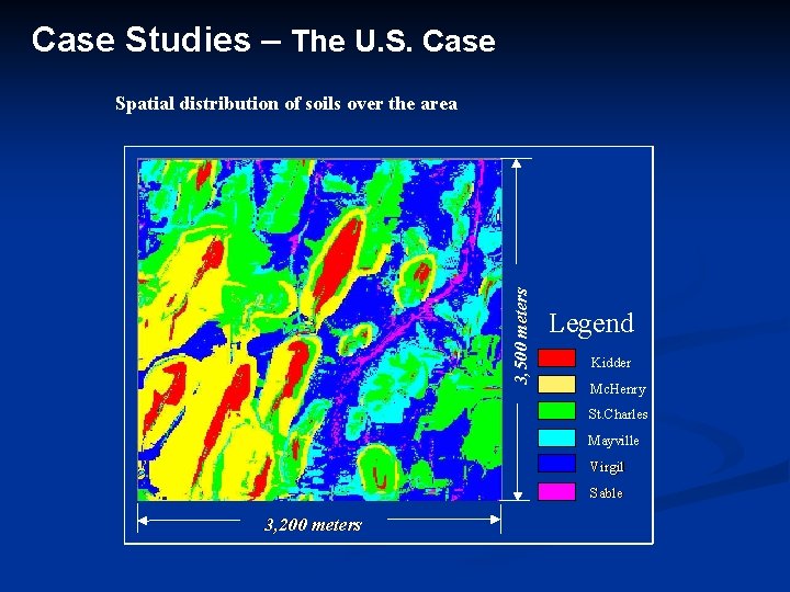
Case Studies – The U. S. Case 3500 meters Study area: A glaciated plain in Wisconsin Soil scientist: John Campbell 3200 meters

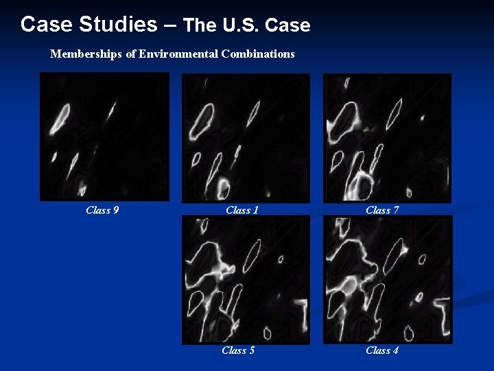
Case Studies – The U. S. Case Memberships of Environmental Combinations Class 9 Class 1 Class 5 Class 7 Class 4

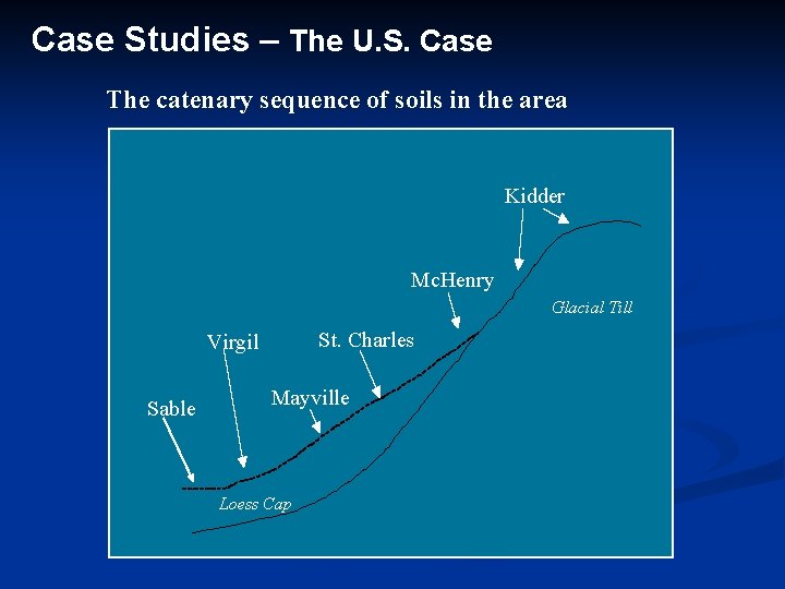
Case Studies – The U. S. Case The catenary sequence of soils in the area Kidder Mc. Henry Glacial Till St. Charles Virgil Sable Mayville Loess Cap

Case Studies – The U. S. Case 3, 500 meters Spatial distribution of soils over the area Legend Kidder Mc. Henry St. Charles Mayville Virgil Sable 3, 200 meters

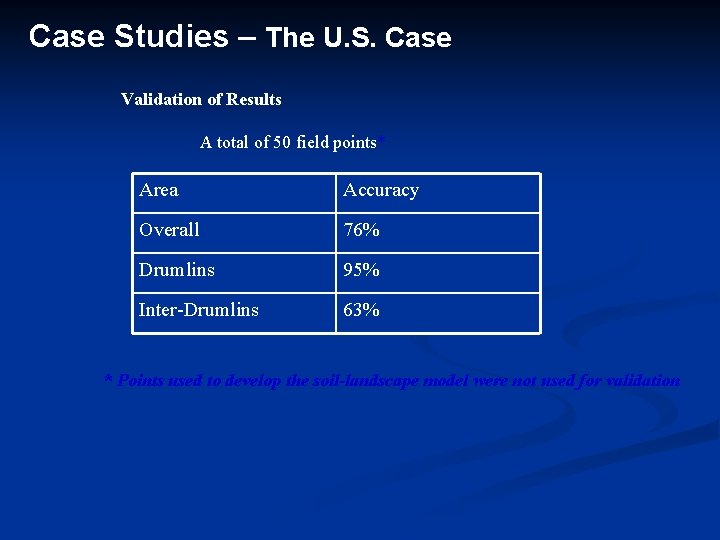
Case Studies – The U. S. Case Validation of Results A total of 50 field points* Area Accuracy Overall 76% Drumlins 95% Inter-Drumlins 63% * Points used to develop the soil-landscape model were not used for validation

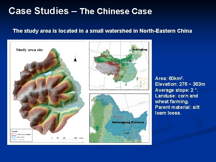
Case Studies – The Chinese Case The study area is located in a small watershed in North-Eastern China Area: 60 km 2. Elevation: 276 ~ 363 m Average slope: 2 °. Landuse: corn and wheat farming. Parent material: silt loam loess.

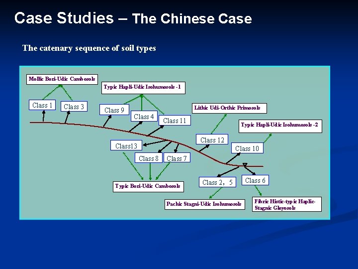
Case Studies – The Chinese Case The catenary sequence of soil types Mollic Bori-Udic Cambosols Typic Hapli-Udic Isohumosols -1 Class 3 Class 9 Lithic Udi-Orthic Primosols Class 4 Class 11 Typic Hapli-Udic Isohumosols -2 Class 13 Class 10 Class 8 Class 7 Typic Bori-Udic Cambosols Class 2，5 Pachic Stagni-Udic Isohumosols Class 6 Fibric Histic-typic Haplic. Stagnic Gleyosols

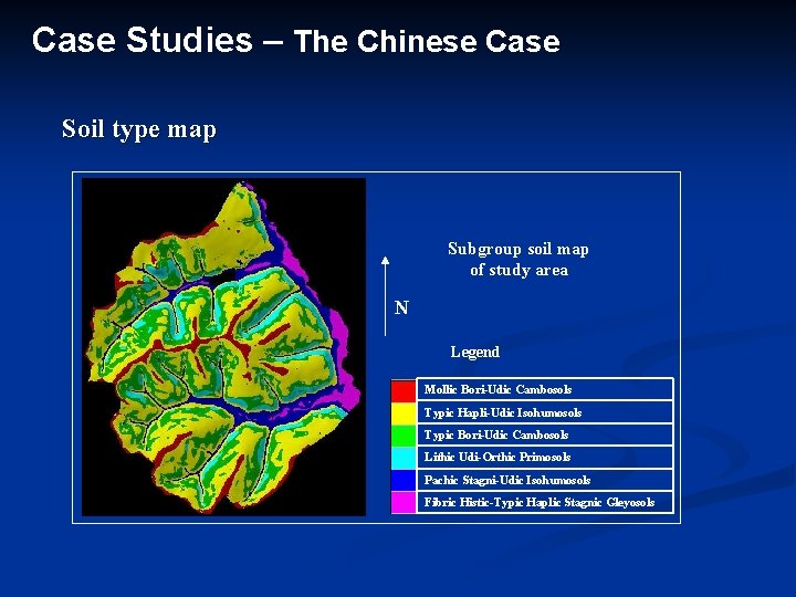
Case Studies – The Chinese Case Soil type map Subgroup soil map of study area N Legend Mollic Bori-Udic Cambosols Typic Hapli-Udic Isohumosols Typic Bori-Udic Cambosols Lithic Udi-Orthic Primosols Pachic Stagni-Udic Isohumosols Fibric Histic-Typic Haplic Stagnic Gleyosols

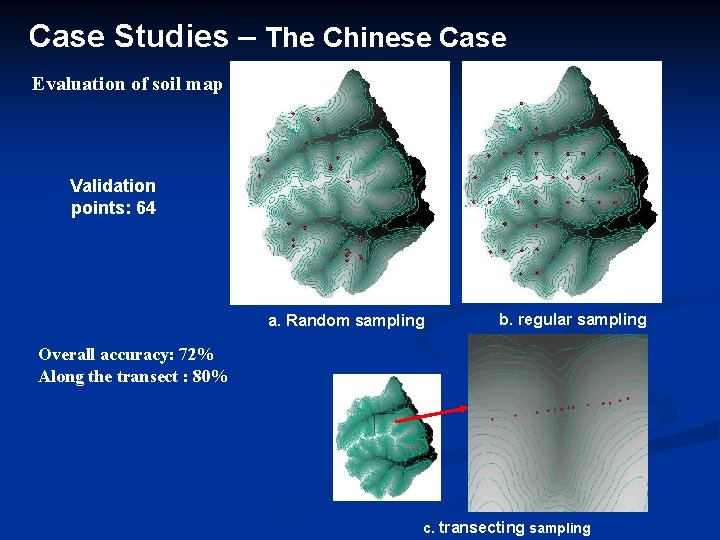
Case Studies – The Chinese Case Evaluation of soil map Validation points: 64 a. Random sampling b. regular sampling Overall accuracy: 72% Along the transect : 80% c. transecting sampling

Summaries The approach does seem to allow us to improve the efficiency of developing soil-landscape model of reasonable quality. The approach seemed to work better in areas with strong relief However, the limitations of fuzzy classification techniques is the key challenge facing this approach

Thank You!