Other ways to detect positive selection Selective sweeps

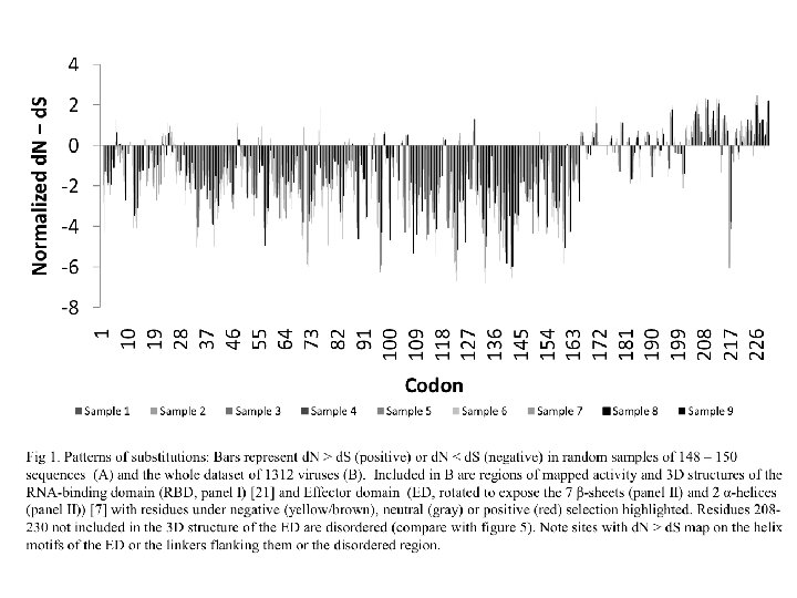
Other ways to detect positive selection Selective sweeps -> fewer alleles present in population (see contributions from Archaic Humans for example) Repeated episodes of positive selection -> high d. N

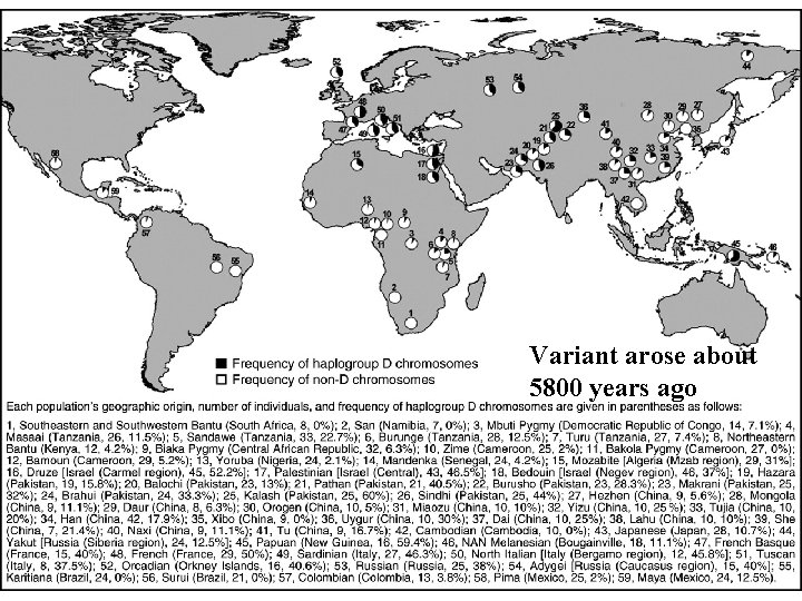
Variant arose about 5800 years ago

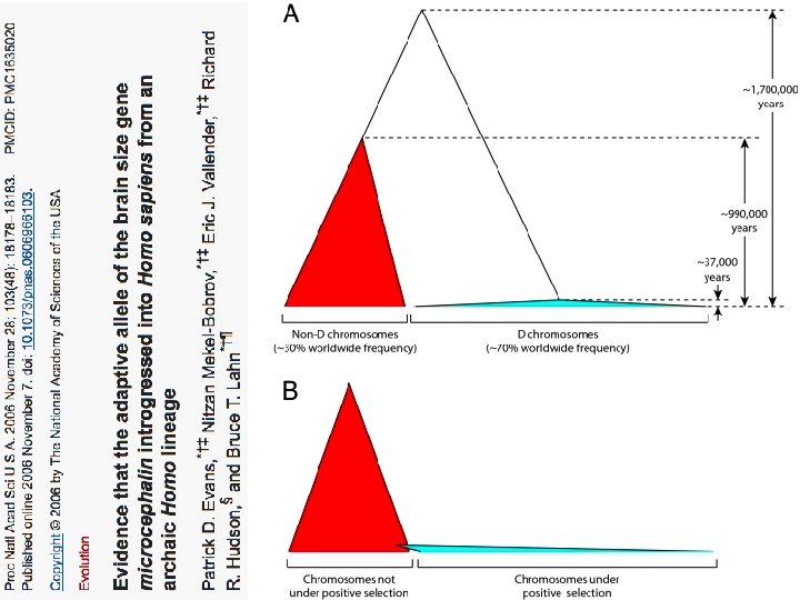
The age of haplogroup D was found to be ~37, 000 years

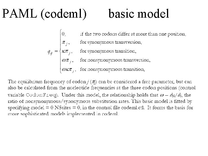
PAML (codeml) the basic model

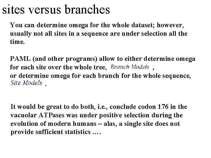
sites versus branches You can determine omega for the whole dataset; however, usually not all sites in a sequence are under selection all the time. PAML (and other programs) allow to either determine omega for each site over the whole tree, , or determine omega for each branch for the whole sequence, . It would be great to do both, i. e. , conclude codon 176 in the vacuolar ATPases was under positive selection during the evolution of modern humans – alas, a single site does not provide sufficient statistics ….

Sites model(s) work great have been shown to work great in few instances. The most celebrated case is the influenza virus HA gene. A talk by Walter Fitch (slides and sound) on the evolution of this molecule is here. This article by Yang et al, 2000 gives more background on ml aproaches to measure omega. The dataset used by Yang et al is here: flu_data. paup.

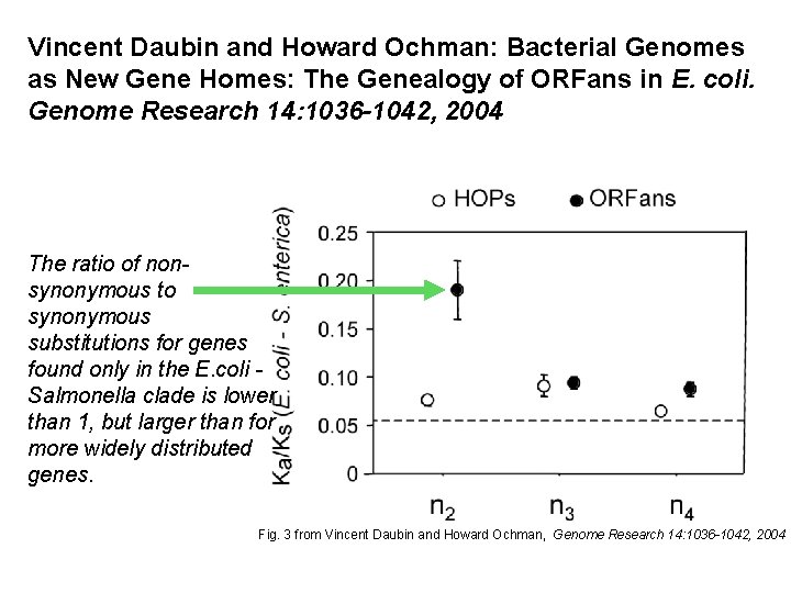
Vincent Daubin and Howard Ochman: Bacterial Genomes as New Gene Homes: The Genealogy of ORFans in E. coli. Genome Research 14: 1036 -1042, 2004 The ratio of nonsynonymous to synonymous substitutions for genes found only in the E. coli Salmonella clade is lower than 1, but larger than for more widely distributed genes. Fig. 3 from Vincent Daubin and Howard Ochman, Genome Research 14: 1036 -1042, 2004

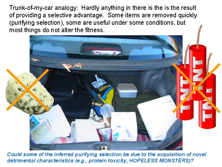
Trunk-of-my-car analogy: Hardly anything in there is the result of providing a selective advantage. Some items are removed quickly (purifying selection), some are useful under some conditions, but most things do not alter the fitness. Could some of the inferred purifying selection be due to the acquisition of novel detrimental characteristics (e. g. , protein toxicity, HOPELESS MONSTERS)?

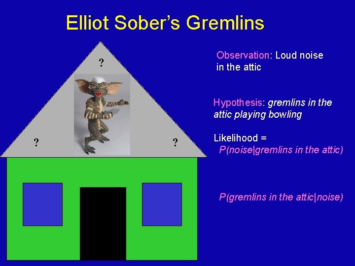
Elliot Sober’s Gremlins Observation: Loud noise in the attic ? Hypothesis: gremlins in the attic playing bowling ? ? Likelihood = P(noise|gremlins in the attic) P(gremlins in the attic|noise)

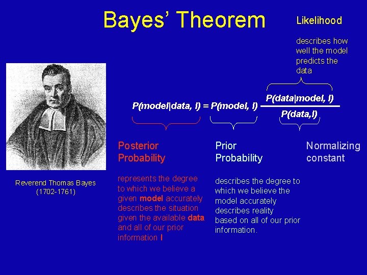
Bayes’ Theorem Likelihood describes how well the model predicts the data P(model|data, I) = P(model, I) Reverend Thomas Bayes (1702 -1761) P(data|model, I) P(data, I) Posterior Probability Prior Probability represents the degree to which we believe a given model accurately describes the situation given the available data and all of our prior information I describes the degree to which we believe the model accurately describes reality based on all of our prior information. Normalizing constant

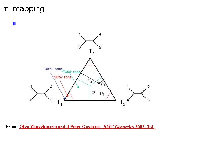
ml mapping From: Olga Zhaxybayeva and J Peter Gogarten BMC Genomics 2002, 3: 4

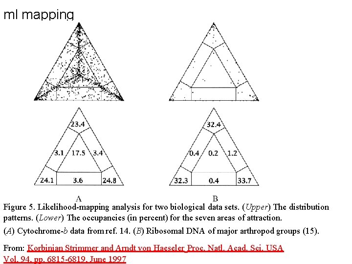
ml mapping Figure 5. Likelihood-mapping analysis for two biological data sets. (Upper) The distribution patterns. (Lower) The occupancies (in percent) for the seven areas of attraction. (A) Cytochrome-b data from ref. 14. (B) Ribosomal DNA of major arthropod groups (15). From: Korbinian Strimmer and Arndt von Haeseler Proc. Natl. Acad. Sci. USA Vol. 94, pp. 6815 -6819, June 1997

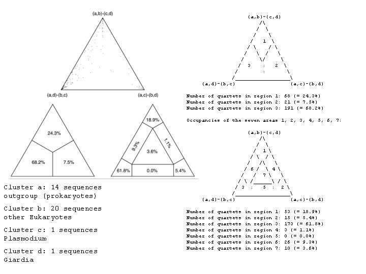
(a, b)-(c, d) / / / 1 / / / / / 3 : 2 / : /_________ (a, d)-(b, c) (a, c)-(b, d) Number of quartets in region 1: 68 (= 24. 3%) Number of quartets in region 2: 21 (= 7. 5%) Number of quartets in region 3: 191 (= 68. 2%) Occupancies of the seven areas 1, 2, 3, 4, 5, 6, 7: Cluster a: 14 sequences outgroup (prokaryotes) Cluster b: 20 sequences other Eukaryotes Cluster c: 1 sequences Plasmodium Cluster d: 1 sequences Giardia (a, b)-(c, d) / / 1 / / / / 6 / 4 / / 7 /______ / 3 : 5 : 2 /_________ (a, d)-(b, c) (a, c)-(b, d) Number Number of of quartets quartets in in region region 1: 2: 3: 4: 5: 6: 7: 53 (= 18. 9%) 15 (= 5. 4%) 173 (= 61. 8%) 3 (= 1. 1%) 0 (= 0. 0%) 26 (= 9. 3%) 10 (= 3. 6%)

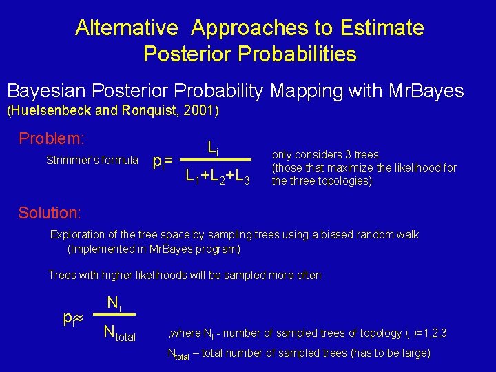
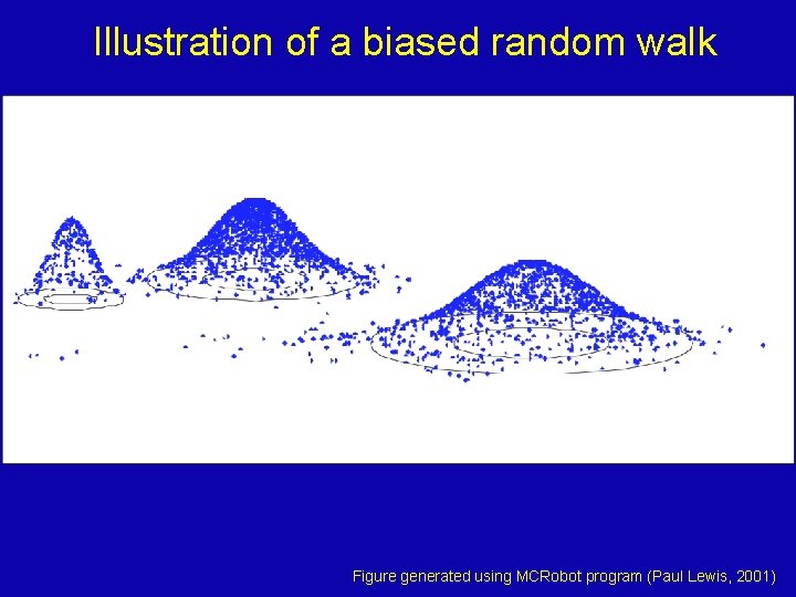
Alternative Approaches to Estimate Posterior Probabilities Bayesian Posterior Probability Mapping with Mr. Bayes (Huelsenbeck and Ronquist, 2001) Problem: Strimmer’s formula p i= Li L 1+L 2+L 3 only considers 3 trees (those that maximize the likelihood for the three topologies) Solution: Exploration of the tree space by sampling trees using a biased random walk (Implemented in Mr. Bayes program) Trees with higher likelihoods will be sampled more often p i Ni Ntotal , where Ni - number of sampled trees of topology i, i=1, 2, 3 Ntotal – total number of sampled trees (has to be large)

Illustration of a biased random walk Figure generated using MCRobot program (Paul Lewis, 2001)

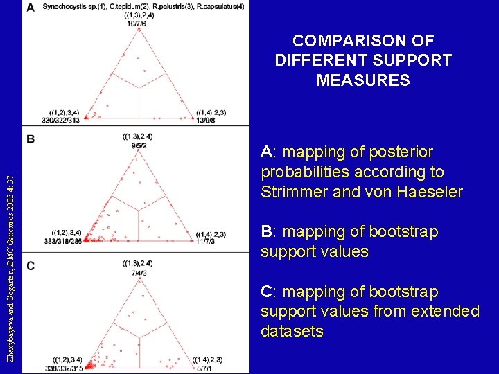
Zhaxybayeva and Gogarten, BMC Genomics 2003 4: 37 COMPARISON OF DIFFERENT SUPPORT MEASURES A: mapping of posterior probabilities according to Strimmer and von Haeseler B: mapping of bootstrap support values C: mapping of bootstrap support values from extended datasets

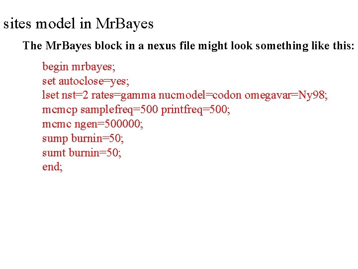
sites model in Mr. Bayes The Mr. Bayes block in a nexus file might look something like this: begin mrbayes; set autoclose=yes; lset nst=2 rates=gamma nucmodel=codon omegavar=Ny 98; mcmcp samplefreq=500 printfreq=500; mcmc ngen=500000; sump burnin=50; sumt burnin=50; end;

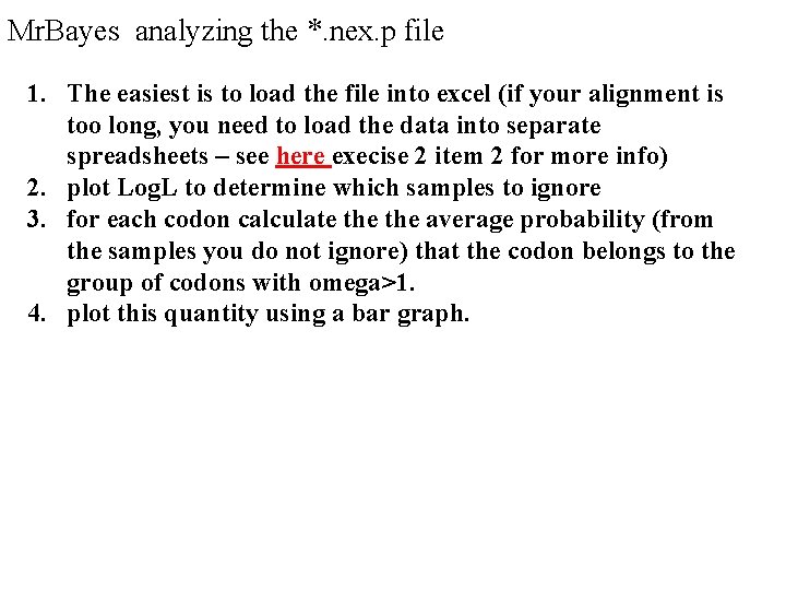
Mr. Bayes analyzing the *. nex. p file 1. The easiest is to load the file into excel (if your alignment is too long, you need to load the data into separate spreadsheets – see here execise 2 item 2 for more info) 2. plot Log. L to determine which samples to ignore 3. for each codon calculate the average probability (from the samples you do not ignore) that the codon belongs to the group of codons with omega>1. 4. plot this quantity using a bar graph.

plot Log. L to determine which samples to ignore the same after rescaling the y-axis

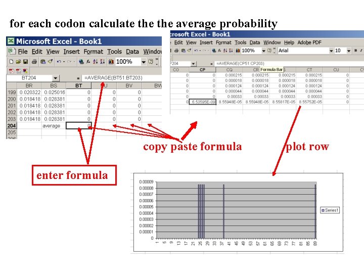
for each codon calculate the average probability copy paste formula enter formula plot row

Mr. Bayes on bbcxrv 1 If you do this for your own data, • run the procedure first for only 50000 generations (takes about 30 minutes) to check that everthing works as expected, • then run the program overnight for at least 500 000 generations. • Especially, if you have a large dataset, do the latter twice and compare the results for consistency. ( I prefer two runs over 500000 generations each over one run over a million generations. ) The preferred way to run mrbayes is to use the command line: >mb Do example on threonly. RS

PAML – codeml – sites model the paml package contains several distinct programs for nucleotides (baseml) protein coding sequences and amino acid sequences (codeml) and to simulate sequences evolution. The input file needs to be in phylip format. By default it assumes a sequential format (e. g. here). If the sequences are interleaved, you need to add an “I” to 6 467 I gi|1613157 -----MSDNDTIVAQ the first line, as in these gi|2212798 example headers: ATPPGRGGVG ILRISGFKAR EVAETVLGKL ----- MSTTDTIVAQ ATPPGRGGVG ILRVSGRAAS EVAHAVLGKL gi|1564003 gi|1560076 gi|2123365 gi|1583936 5 855 I human goat-cow rabbit rat marsupial 1 GTG CTG TCT. . . C. . G 61 GCT. . G. . . C GGC. . A. . . T GAG. CT. . . A. CC MALIQSCSGN -----MN-------MSQRS TMTTDTIVAQ QAATETIVAI -ALPSTIVAI TKMGDTIAAI ATAPGRGGVG ATAQGRGGVG ATAAGTGGIG ATASGAAGIG IIRVSGPLAA IVRVSGPLAG IVRLSGPQSV IIRLSGSLIK HVAQTVTGRT QMAVAVSGRQ QIAAALGIAG TIATGLGMTT PKPRYADYLP LRPRYAEYLP LKARHAHYGP LQSRHARYAR LRPRYAHYTR FKDADGSVLD FKDVDGSTLD FTDEDGQQLD FLDAGGQVID FRDAQGEVID FLDVQDEVID QGIALWFPGP QGIALYFPGP QGIALFFPNP EGLSLYFPGP DGIAVWFPAP DGLALWFPAP NSFTGEDVLE HSFTGEDVLE NSFTGEDVLE HSFTGEEVVE HSFTGEDVLE LQGHGGPVIL LQGHGGPVVM LQGHGGPVVL LQGHGSPVLL LQGHGSPLLL CCT G. C. . C G. A GA. GCC. . . T. AT. . T GAC. . . AAG. . . . A. . . ACC T. . T AAC. . T. . . C. . GTC. . . A. . G AAG. . . A GCC. . . A. T AA. . GCC. . . TG. AT. TGG. . . GGC. . AA. . G. . T AAG. . . GTT. . . A. C A. . G GGC. . . . T. . A GCG. GC AGC. GC CAC A. . . . T. . . TAT. . . C GGT. . C. CA GCG. . A. . C. A. . . T GAG. . . A GCC. . T. . . . T CTG. . . . A. . T GAG. . . CC AGG. . . A ATG. . CC TTC. . . CTG. . . T. . GCT. . C TCC AG. G. . . TTC. . . CCC. . . ACC. . . T ACC. . . AAG. . . A

PAML – codeml – sites model (cont. ) the program is invoked by typing codeml followed by the name of a control file that tells the program what to do. paml can be used to find the maximum likelihood tree, however, the program is rather slow. Phyml is a better choice to find the tree, which then can be used as a user tree. An example for a codeml. ctl file is codeml. hv 1. sites. ctl This file directs codeml to run three different models: one with an omega fixed at 1, a second where each site can be either have an omega between 0 and 1, or an omega of 1, and third a model that uses three omegas as described before for Mr. Bayes. The output is written into a file called Hv 1. sites. codeml_out (as directed by the control file). Point out log likelihoods and estimated parameter line (kappa and omegas) Additional useful information is in the rst file generated by the codeml Discuss overall result.

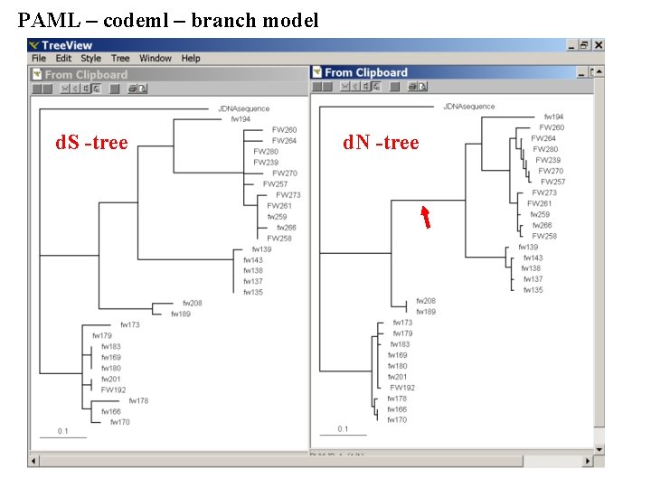
PAML – codeml – branch model For the same dataset to estimate the d. N/d. S ratios for individual branches, you could use this file codeml. hv 1. branches. ctl as control file. The output is written, as directed by the control file, into a file called Hv 1. branch. codeml_out A good way to check for episodes with plenty of non-synonymous substitutions is to compare the dn and ds trees. Also, it might be a good idea to repeat the analyses on parts of the sequence (using the same tree). In this case the sequences encode a family of spider toxins that include the mature toxin, a propeptide and a signal sequence (see here for more information). Bottom line: one needs plenty of sequences to detect positive selection.

PAML – codeml – branch model d. S -tree d. N -tree

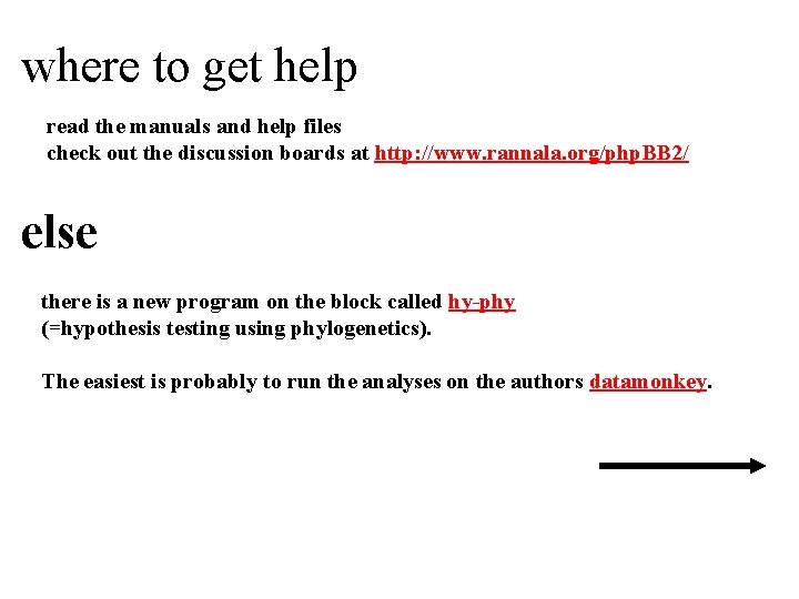
where to get help read the manuals and help files check out the discussion boards at http: //www. rannala. org/php. BB 2/ else there is a new program on the block called hy-phy (=hypothesis testing using phylogenetics). The easiest is probably to run the analyses on the authors datamonkey.

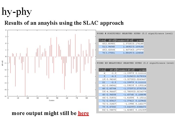
hy-phy Results of an anaylsis using the SLAC approach more output might still be here

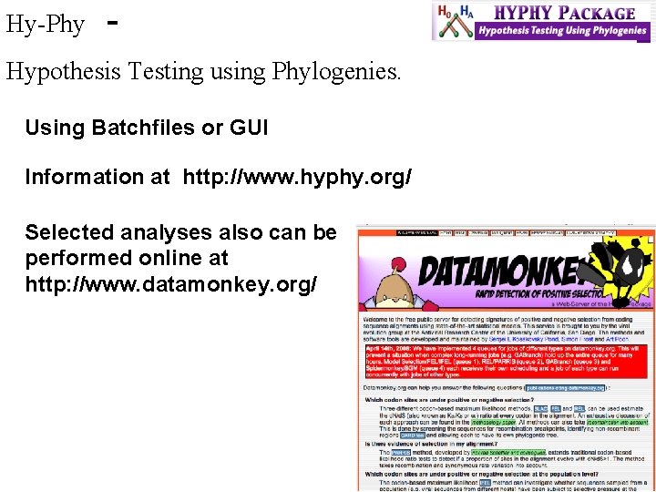
Hy-Phy - Hypothesis Testing using Phylogenies. Using Batchfiles or GUI Information at http: //www. hyphy. org/ Selected analyses also can be performed online at http: //www. datamonkey. org/

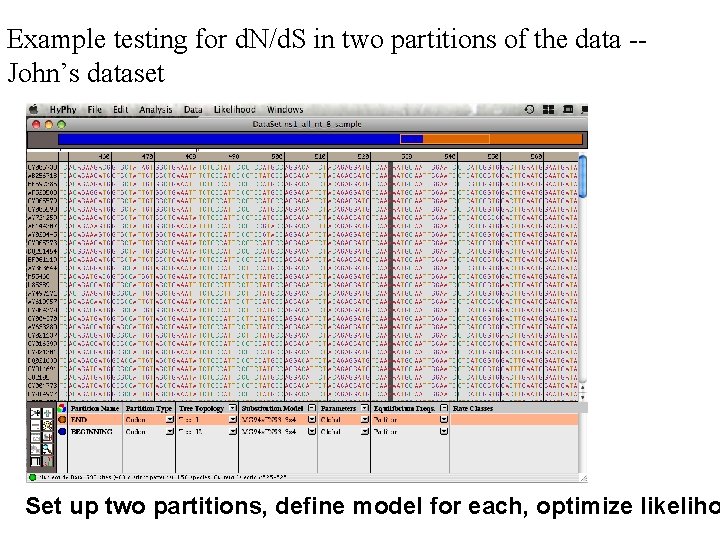
Example testing for d. N/d. S in two partitions of the data -John’s dataset Set up two partitions, define model for each, optimize likeliho

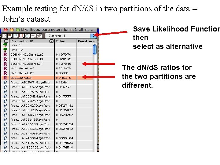
Example testing for d. N/d. S in two partitions of the data -John’s dataset Save Likelihood Function then select as alternative The d. N/d. S ratios for the two partitions are different.

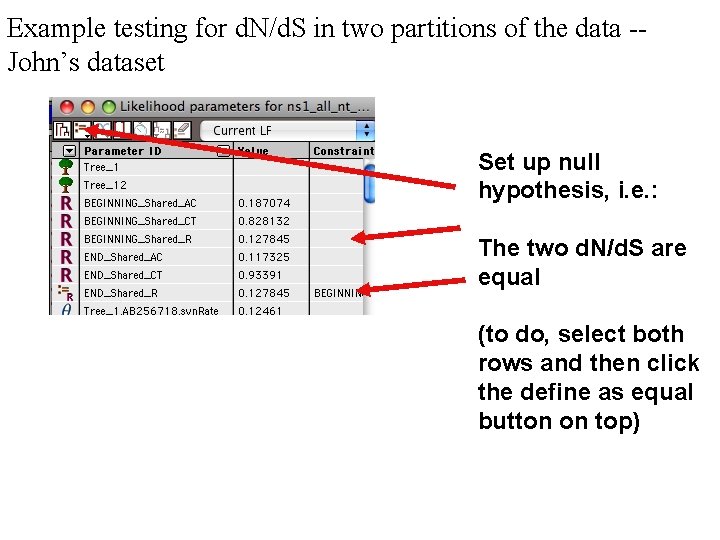
Example testing for d. N/d. S in two partitions of the data -John’s dataset Set up null hypothesis, i. e. : The two d. N/d. S are equal (to do, select both rows and then click the define as equal button on top)

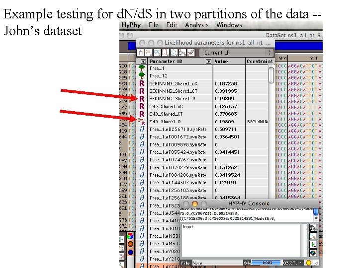
Example testing for d. N/d. S in two partitions of the data -John’s dataset

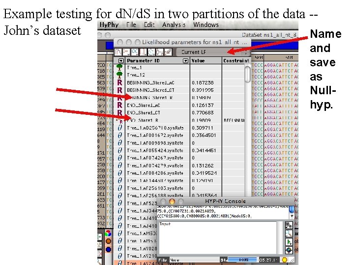
Example testing for d. N/d. S in two partitions of the data -John’s dataset Name and save as Nullhyp.

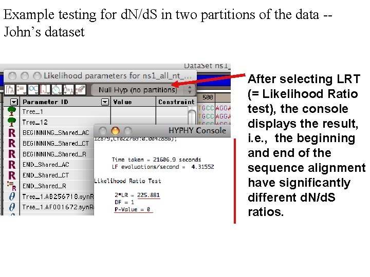
Example testing for d. N/d. S in two partitions of the data -John’s dataset After selecting LRT (= Likelihood Ratio test), the console displays the result, i. e. , the beginning and end of the sequence alignment have significantly different d. N/d. S ratios.

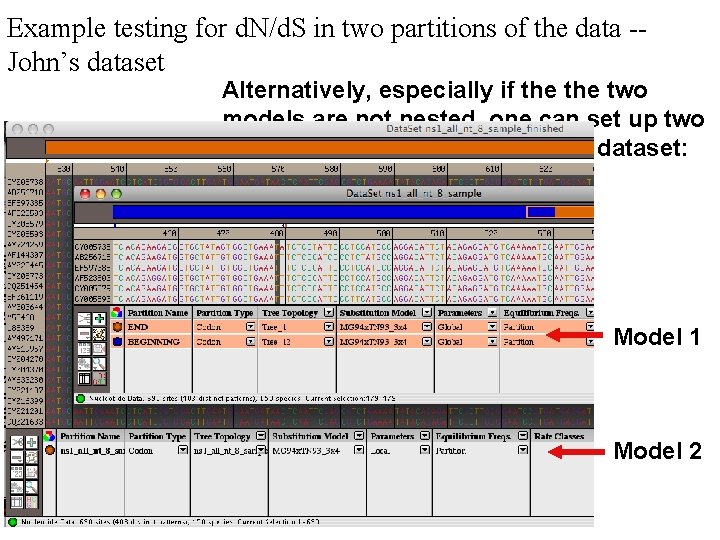
Example testing for d. N/d. S in two partitions of the data -John’s dataset Alternatively, especially if the two models are not nested, one can set up two different windows with the same dataset: Model 1 Model 2

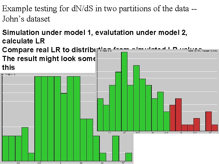
Example testing for d. N/d. S in two partitions of the data -John’s dataset Simulation under model 1, evalutation under model 2, calculate LR Compare real LR to distribution from simulated LR values. The result might look something like this or this