OST Chapter 3 Part 1 Tactical planning Layout

OST: Chapter 3 (Part 1) Tactical planning: Layout Fixed-position layout Job shop production 1 (LAP)

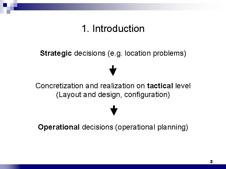
1. Introduction Strategic decisions (e. g. location problems) Concretization and realization on tactical level (Layout and design, configuration) Operational decisions (operational planning) 2

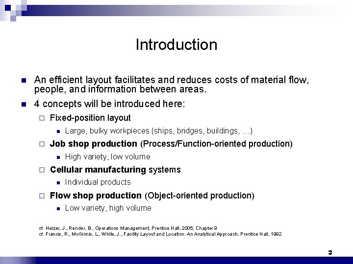
Introduction n n An efficient layout facilitates and reduces costs of material flow, people, and information between areas. 4 concepts will be introduced here: ¨ Fixed-position layout n ¨ Job shop production (Process/Function-oriented production) n ¨ High variety, low volume Cellular manufacturing systems n ¨ Large, bulky workpieces (ships, bridges, buildings, …) Individual products Flow shop production (Object-oriented production) n Low variety, high volume cf. Heizer, J. , Render, B. , Operations Management, Prentice Hall, 2006, Chapter 9 cf. Francis, R. , Mc. Ginnis, L. , White, J. , Facility Layout and Location: An Analytical Approach, Prentice Hall, 1992 3

Introduction / Example: Production and assembly of 4 parts (A, B, C, D) n ¨ ¨ n A: saw -> turn -> mill -> drill B: saw -> mill -> drill -> paint C: grind -> mill -> drill -> paint D: weld -> grind -> turn -> drill Minimum equipment: ¨ ¨ ¨ ¨ 1 weld 1 grind 1 saw 1 turn 2 mills 2 drills 1 paint Equipment requirements Part Weld Grind Saw Turn Mill Drill Paint A - - 0. 5 0. 3 0. 2 - B - - 0. 4 - 0. 5 0. 3 0. 2 C - 0. 4 - - 0. 3 0. 5 0. 3 D 0. 3 0. 5 - 0. 3 - 0. 2 - cf. Heizer, J. , Render, B. , Operations Management, Prentice Hall, 2006, Chapter 9 cf. Francis, R. , Mc. Ginnis, L. , White, J. , Facility Layout and Location: An Analytical Approach, Prentice Hall, 1992 4

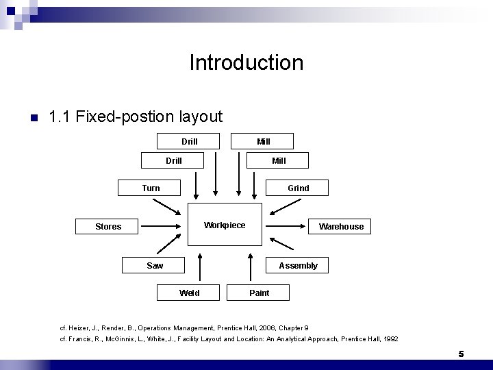
Introduction n 1. 1 Fixed-postion layout Drill Mill Turn Grind Workpiece Stores Warehouse Saw Assembly Weld Paint cf. Heizer, J. , Render, B. , Operations Management, Prentice Hall, 2006, Chapter 9 cf. Francis, R. , Mc. Ginnis, L. , White, J. , Facility Layout and Location: An Analytical Approach, Prentice Hall, 1992 5

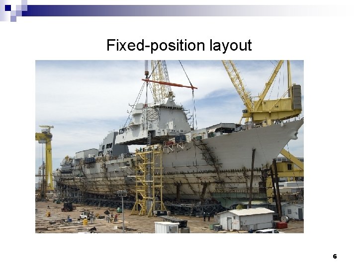
Fixed-position layout http: //business. mrwood. com. au/unit 3/opstrat 1. asp 6

Introduction n 1. 2 Job shop layout cf. Heizer, J. , Render, B. , Operations Management, Prentice Hall, 2006, Chapter 9 cf. Francis, R. , Mc. Ginnis, L. , White, J. , Facility Layout and Location: An Analytical Approach, Prentice Hall, 1992 7

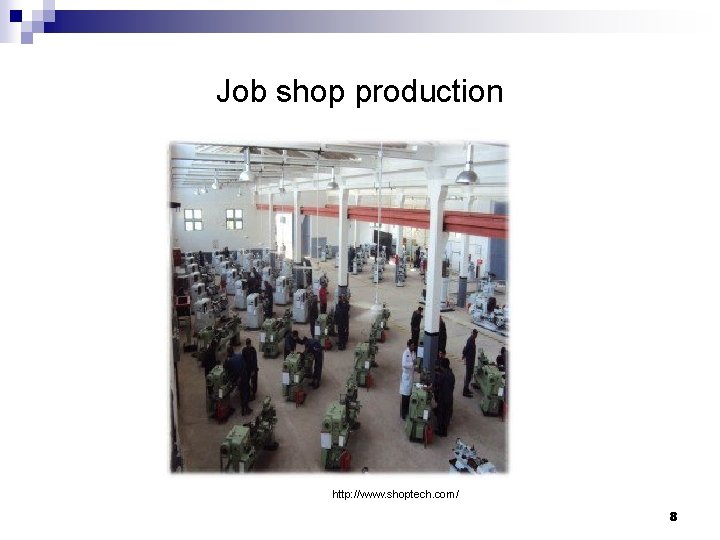
Job shop production http: //www. shoptech. com/ 8

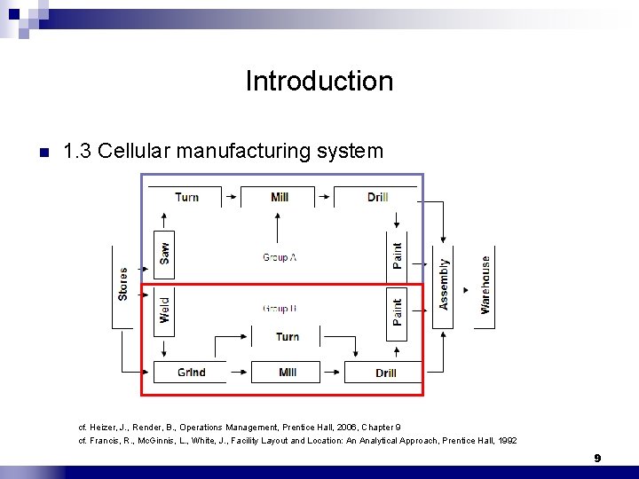
Introduction n 1. 3 Cellular manufacturing system cf. Heizer, J. , Render, B. , Operations Management, Prentice Hall, 2006, Chapter 9 cf. Francis, R. , Mc. Ginnis, L. , White, J. , Facility Layout and Location: An Analytical Approach, Prentice Hall, 1992 9

Cellular manufacturing system http: //www. tpslean. com/glossary/cellmfgdef. htm (c) Prof. Richard F. Hartl

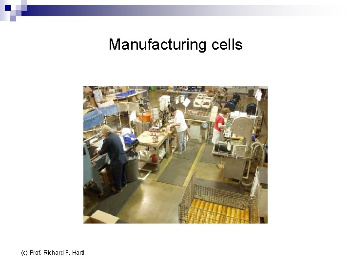
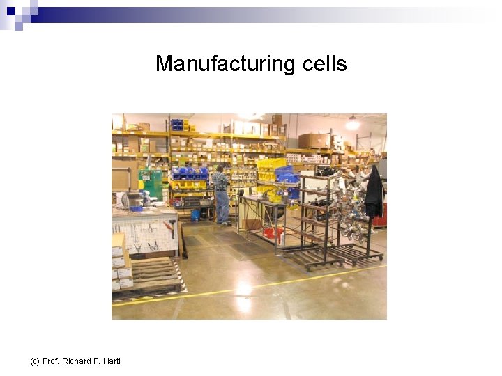
Manufacturing cells (c) Prof. Richard F. Hartl

Manufacturing cells (c) Prof. Richard F. Hartl

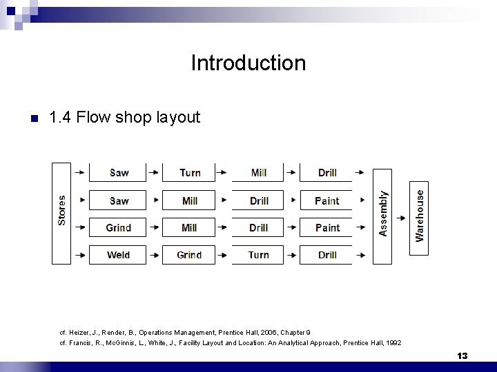
Introduction n 1. 4 Flow shop layout cf. Heizer, J. , Render, B. , Operations Management, Prentice Hall, 2006, Chapter 9 cf. Francis, R. , Mc. Ginnis, L. , White, J. , Facility Layout and Location: An Analytical Approach, Prentice Hall, 1992 13

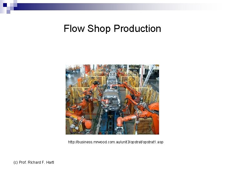
Flow Shop Production http: //business. mrwood. com. au/unit 3/opstrat 1. asp (c) Prof. Richard F. Hartl

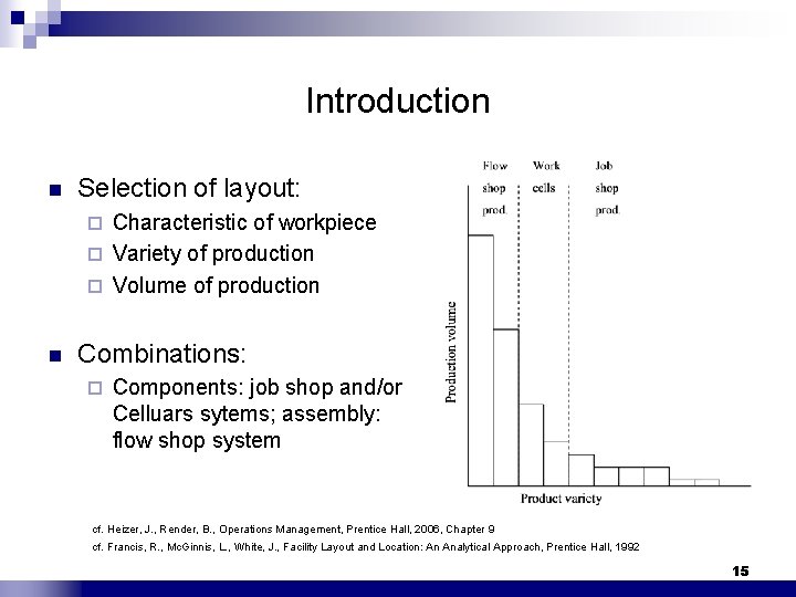
Introduction n Selection of layout: Characteristic of workpiece ¨ Variety of production ¨ Volume of production ¨ n Combinations: ¨ Components: job shop and/or Celluars sytems; assembly: flow shop system cf. Heizer, J. , Render, B. , Operations Management, Prentice Hall, 2006, Chapter 9 cf. Francis, R. , Mc. Ginnis, L. , White, J. , Facility Layout and Location: An Analytical Approach, Prentice Hall, 1992 15

2. Fixed-Position Layout n Workpiece too large or cumbersome to be moved trough its processing steps -> processes are brought to the product rather than otherwise. n Processes are arranged in the right sequence around the workpiece n Right processes at the workpiece at the right location in the right time cf. Heizer, J. , Render, B. , Operations Management, Prentice Hall, 2006, Chapter 9 cf. Francis, R. , Mc. Ginnis, L. , White, J. , Facility Layout and Location: An Analytical Approach, Prentice Hall, 1992 16

Fixed-position layout n Advantages: Material movement is reduced. ¨ Promotes job enlargement by allowing individuals or teams to perform the “whole job”. ¨ Highly flexible; can accommodate changes in product design, product mix, and production volume. ¨ Independence of production centres allows scheduling to achieve minimum total production time. ¨ cf. Heizer, J. , Render, B. , Operations Management, Prentice Hall, 2006, Chapter 9 cf. Francis, R. , Mc. Ginnis, L. , White, J. , Facility Layout and Location: An Analytical Approach, Prentice Hall, 1992 17

Fixed-position layout n Limitations: ¨ ¨ ¨ Increased movement of personnel and equipment. Equipment duplication may occur. Higher skill requirements for personnel. General supervision required. Cumbersome and costly positioning of material and machinery. Low equipment utilization. cf. Heizer, J. , Render, B. , Operations Management, Prentice Hall, 2006, Chapter 9 cf. Francis, R. , Mc. Ginnis, L. , White, J. , Facility Layout and Location: An Analytical Approach, Prentice Hall, 1992 18

3. Job Shop Production n n n High variety – low volume Rapid changes in mix or volume „In-between conditions“ Collection of processing departments or cells Each containing a collection of machines processing similiar operations Each product (group) undergoes a different sequence of operations Different products have different material flows and are moved from one department to another in the appropriate sequence. High degree of interdepartmental flow cf. Heizer, J. , Render, B. , Operations Management, Prentice Hall, 2006, Chapter 9 cf. Francis, R. , Mc. Ginnis, L. , White, J. , Facility Layout and Location: An Analytical Approach, Prentice Hall, 1992 19

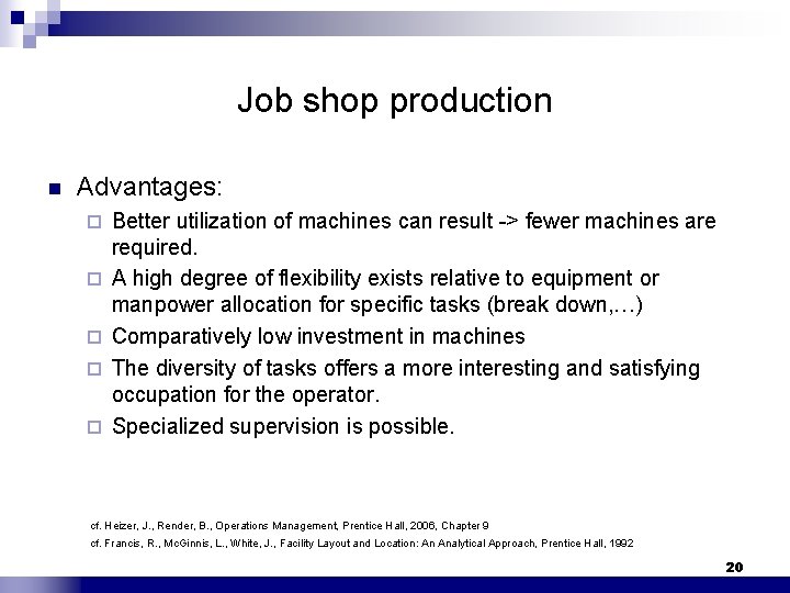
Job shop production n Advantages: ¨ ¨ ¨ Better utilization of machines can result -> fewer machines are required. A high degree of flexibility exists relative to equipment or manpower allocation for specific tasks (break down, …) Comparatively low investment in machines The diversity of tasks offers a more interesting and satisfying occupation for the operator. Specialized supervision is possible. cf. Heizer, J. , Render, B. , Operations Management, Prentice Hall, 2006, Chapter 9 cf. Francis, R. , Mc. Ginnis, L. , White, J. , Facility Layout and Location: An Analytical Approach, Prentice Hall, 1992 20

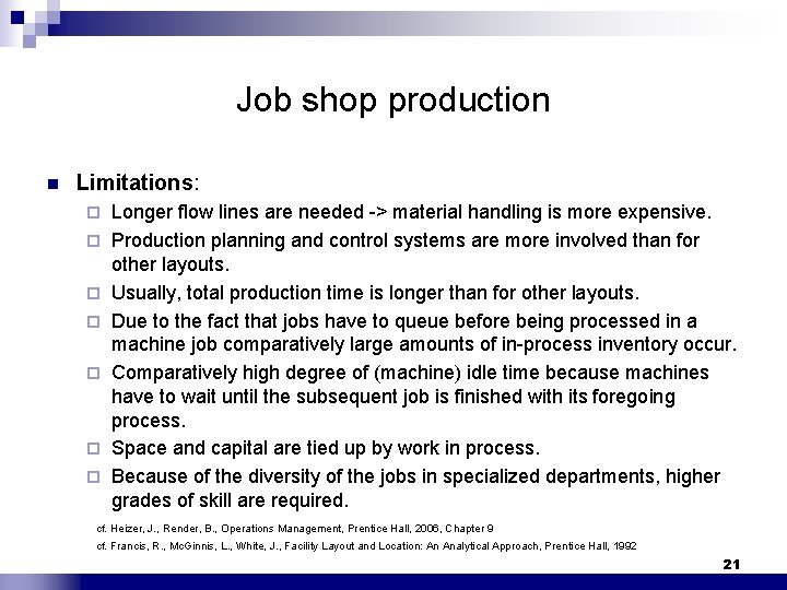
Job shop production n Limitations: ¨ ¨ ¨ ¨ Longer flow lines are needed -> material handling is more expensive. Production planning and control systems are more involved than for other layouts. Usually, total production time is longer than for other layouts. Due to the fact that jobs have to queue before being processed in a machine job comparatively large amounts of in-process inventory occur. Comparatively high degree of (machine) idle time because machines have to wait until the subsequent job is finished with its foregoing process. Space and capital are tied up by work in process. Because of the diversity of the jobs in specialized departments, higher grades of skill are required. cf. Heizer, J. , Render, B. , Operations Management, Prentice Hall, 2006, Chapter 9 cf. Francis, R. , Mc. Ginnis, L. , White, J. , Facility Layout and Location: An Analytical Approach, Prentice Hall, 1992 21

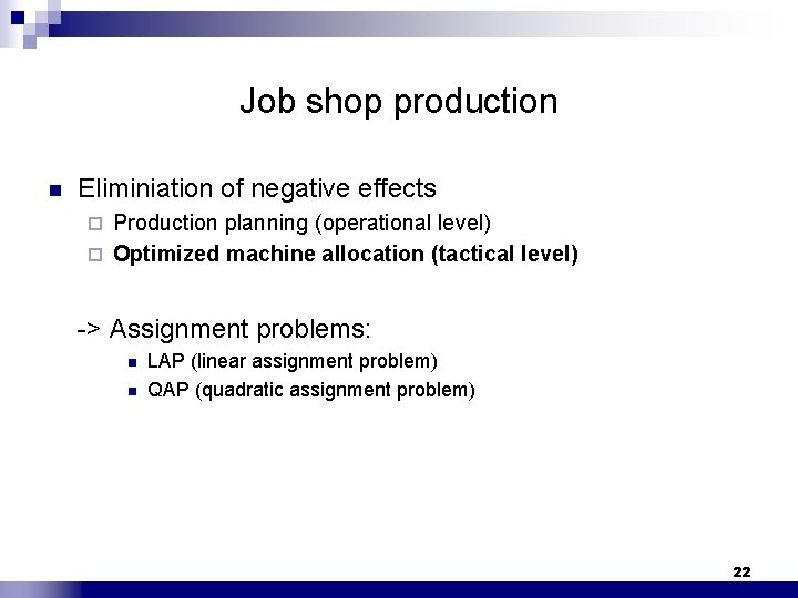
Job shop production n Eliminiation of negative effects Production planning (operational level) ¨ Optimized machine allocation (tactical level) ¨ -> Assignment problems: n n LAP (linear assignment problem) QAP (quadratic assignment problem) 22

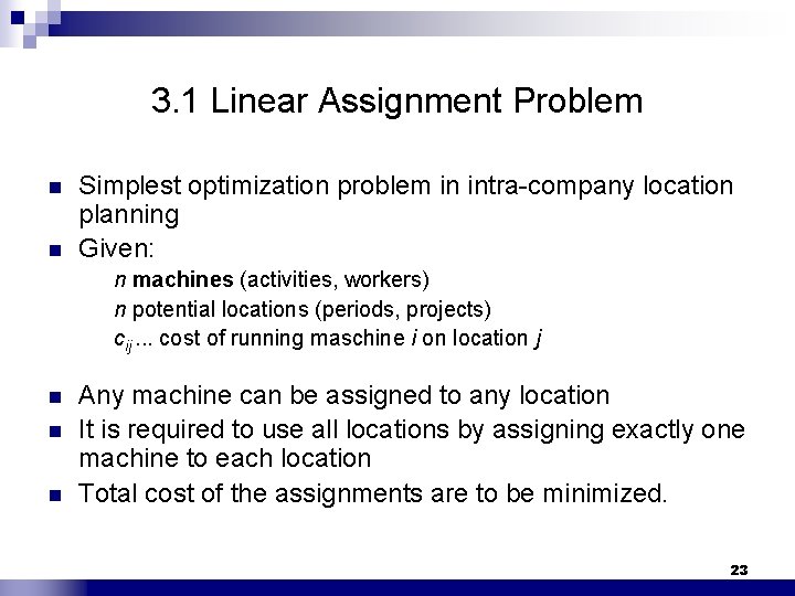
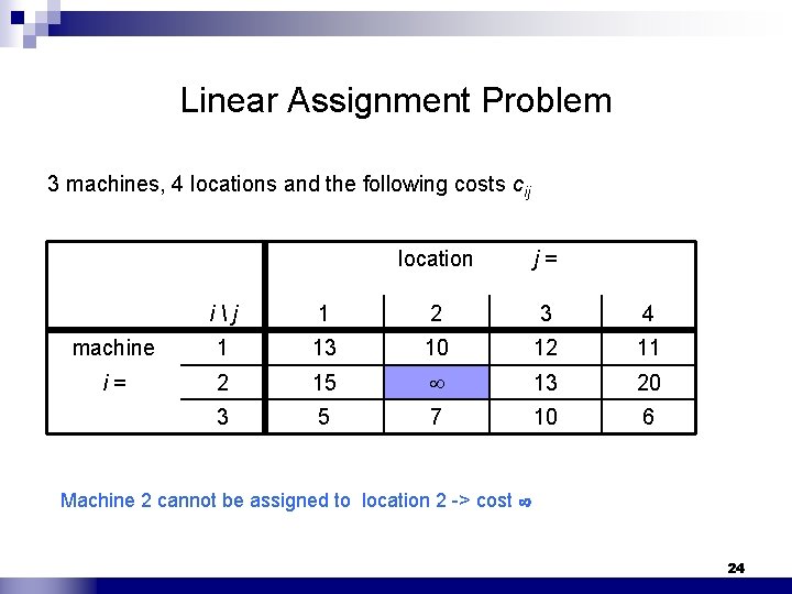
3. 1 Linear Assignment Problem n n Simplest optimization problem in intra-company location planning Given: n machines (activities, workers) n potential locations (periods, projects) cij. . . cost of running maschine i on location j n n n Any machine can be assigned to any location It is required to use all locations by assigning exactly one machine to each location Total cost of the assignments are to be minimized. 23

Linear Assignment Problem 3 machines, 4 locations and the following costs cij location j= ij 1 2 3 4 machine 1 13 10 12 11 i = 2 15 13 20 3 5 7 10 6 Machine 2 cannot be assigned to location 2 -> cost 24

Linear Assignment Problem n If number of locations ≠ number of machines: ¨ Add dummymachines (-rows) or dummylocations (-columns) with costs 0 (this is always possible) locations j= ij 1 2 3 4 machine 1 13 10 12 11 i = 2 15 13 20 3 5 7 10 6 4 0 0 dummy Location with dummy machine -> location stays empty 25

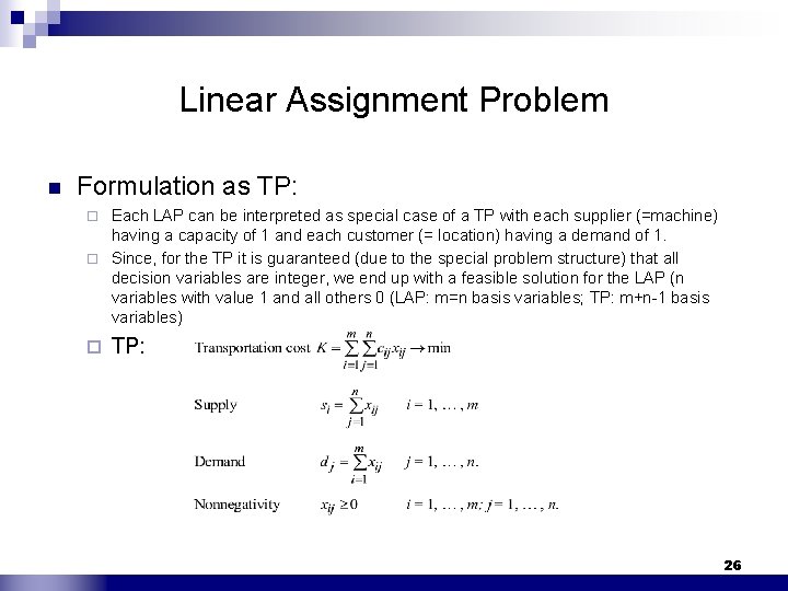
Linear Assignment Problem n Formulation as TP: Each LAP can be interpreted as special case of a TP with each supplier (=machine) having a capacity of 1 and each customer (= location) having a demand of 1. ¨ Since, for the TP it is guaranteed (due to the special problem structure) that all decision variables are integer, we end up with a feasible solution for the LAP (n variables with value 1 and all others 0 (LAP: m=n basis variables; TP: m+n-1 basis variables) ¨ ¨ TP: 26

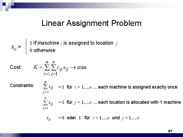
Linear Assignment Problem 1 if maschine i is assigned to location j xij = 0 otherwise Cost: Constraints: = 1 für i = 1, . . . , n. . . each machine is assigned exactly once = 1 für j = 1, . . . , n. . . each location is allocated with 1 machine = 0 oder 1 für i = 1, . . . , n und j = 1, . . . , n 27

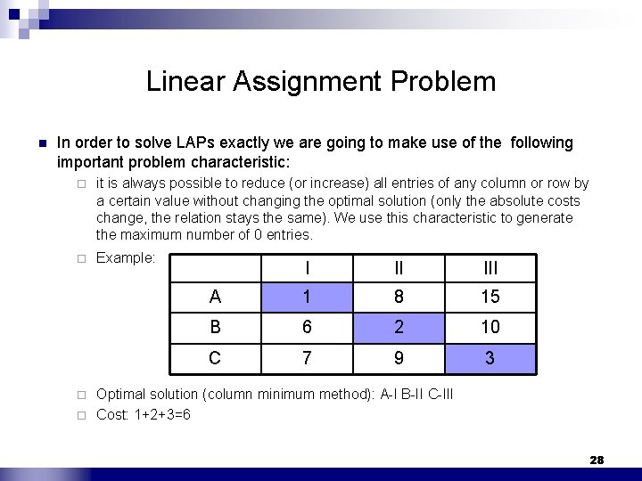
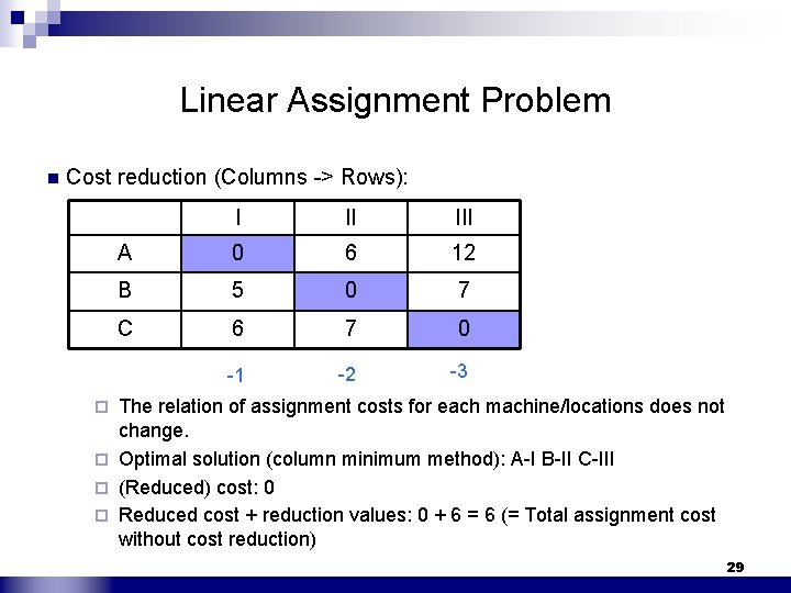
Linear Assignment Problem n In order to solve LAPs exactly we are going to make use of the following important problem characteristic: ¨ it is always possible to reduce (or increase) all entries of any column or row by a certain value without changing the optimal solution (only the absolute costs change, the relation stays the same). We use this characteristic to generate the maximum number of 0 entries. ¨ Example: I II III A 1 8 15 B 6 2 10 C 7 9 3 Optimal solution (column minimum method): A-I B-II C-III ¨ Cost: 1+2+3=6 ¨ 28

Linear Assignment Problem n Cost reduction (Columns -> Rows): I II III A 0 6 12 B 5 0 7 C 6 7 0 -1 -2 -3 The relation of assignment costs for each machine/locations does not change. ¨ Optimal solution (column minimum method): A-I B-II C-III ¨ (Reduced) cost: 0 ¨ Reduced cost + reduction values: 0 + 6 = 6 (= Total assignment cost without cost reduction) ¨ 29

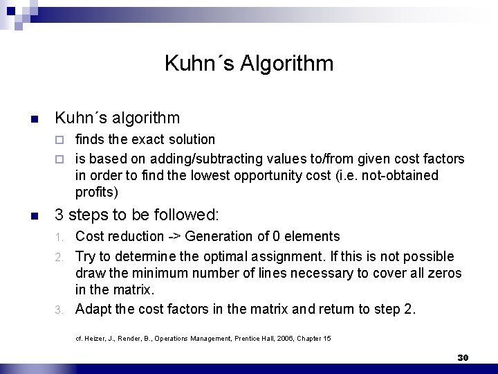
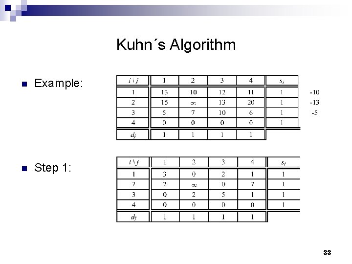
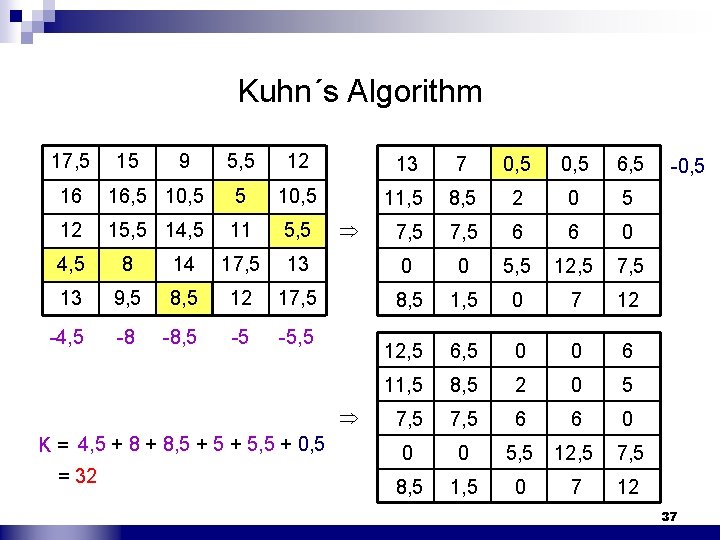
Kuhn´s Algorithm n Kuhn´s algorithm finds the exact solution ¨ is based on adding/subtracting values to/from given cost factors in order to find the lowest opportunity cost (i. e. not-obtained profits) ¨ n 3 steps to be followed: Cost reduction -> Generation of 0 elements 2. Try to determine the optimal assignment. If this is not possible draw the minimum number of lines necessary to cover all zeros in the matrix. 3. Adapt the cost factors in the matrix and return to step 2. 1. cf. Heizer, J. , Render, B. , Operations Management, Prentice Hall, 2006, Chapter 15 30

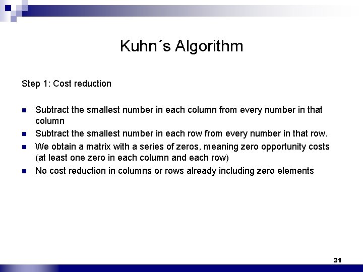
Kuhn´s Algorithm Step 1: Cost reduction n n Subtract the smallest number in each column from every number in that column Subtract the smallest number in each row from every number in that row. We obtain a matrix with a series of zeros, meaning zero opportunity costs (at least one zero in each column and each row) No cost reduction in columns or rows already including zero elements 31

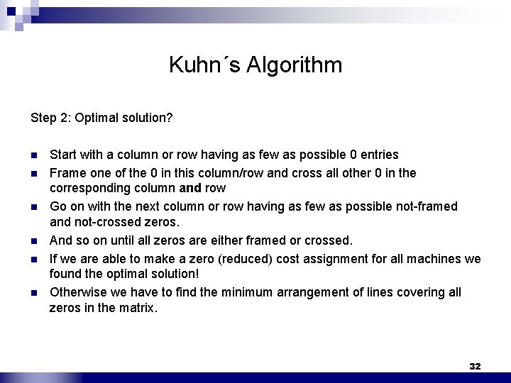
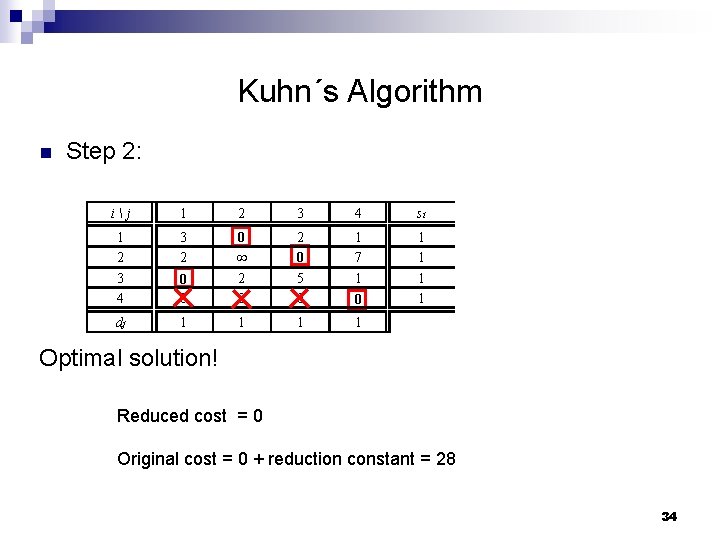
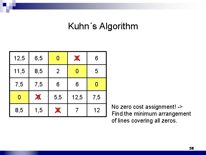
Kuhn´s Algorithm Step 2: Optimal solution? n n n Start with a column or row having as few as possible 0 entries Frame one of the 0 in this column/row and cross all other 0 in the corresponding column and row Go on with the next column or row having as few as possible not-framed and not-crossed zeros. And so on until all zeros are either framed or crossed. If we are able to make a zero (reduced) cost assignment for all machines we found the optimal solution! Otherwise we have to find the minimum arrangement of lines covering all zeros in the matrix. 32

Kuhn´s Algorithm n Example: n Step 1: 33

Kuhn´s Algorithm n Step 2: ij 1 2 3 4 si 1 2 3 4 3 2 0 0 0 2 0 5 0 1 7 1 0 1 1 dj 1 1 Optimal solution! Reduced cost = 0 Original cost = 0 + reduction constant = 28 34

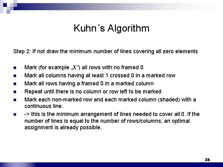
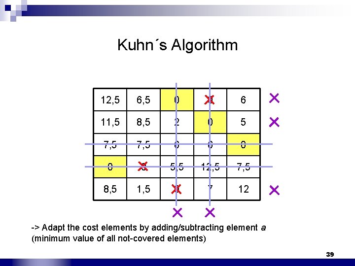
Kuhn´s Algorithm Step 2: If not draw the minimum number of lines covering all zero elements n n n Mark (for example „X“) all rows with no framed 0 Mark all columns having at least 1 crossed 0 in a marked row Mark all rows having a framed 0 in a marked column Repeat until there is no column or row left to be marked Mark each non-marked row and each marked column (shaded) with a continuous line. -> this is the minimum arrangement of lines needed to cover all 0. If the number of lines is equal to the number of rows/columns, an optimal assignment is already possible. 35

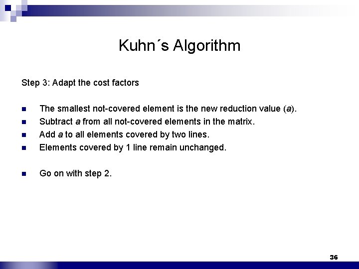
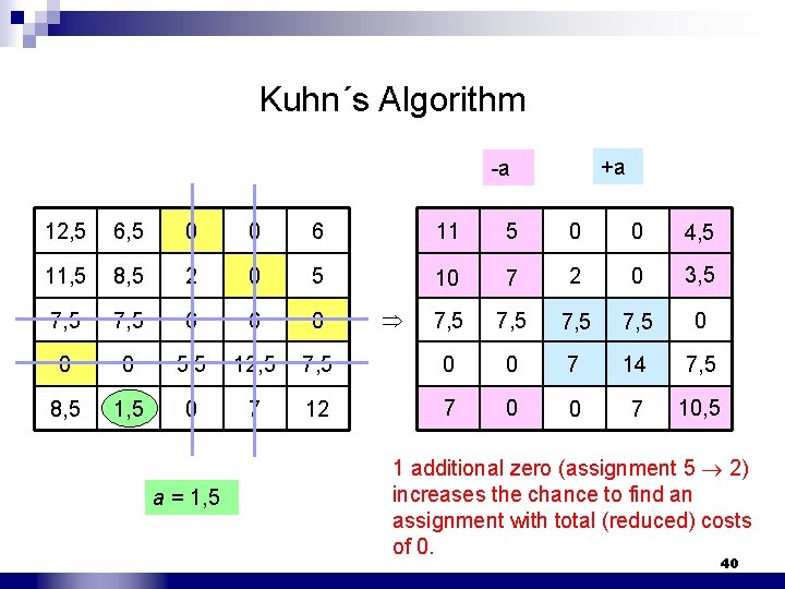
Kuhn´s Algorithm Step 3: Adapt the cost factors n The smallest not-covered element is the new reduction value (a). Subtract a from all not-covered elements in the matrix. Add a to all elements covered by two lines. Elements covered by 1 line remain unchanged. n Go on with step 2. n n n 36

Kuhn´s Algorithm 17, 5 15 9 5, 5 12 13 7 0, 5 6, 5 11, 5 8, 5 2 0 5 7, 5 6 6 0 16 16, 5 10, 5 12 15, 5 14, 5 11 5, 5 4, 5 8 14 17, 5 13 0 0 5, 5 12, 5 7, 5 13 9, 5 8, 5 12 17, 5 8, 5 1, 5 0 7 12 -4, 5 -8 -8, 5 -5 -5, 5 12, 5 6, 5 0 0 6 11, 5 8, 5 2 0 5 7, 5 6 6 0 0 0 5, 5 12, 5 7, 5 8, 5 1, 5 0 7 12 K = 4, 5 + 8, 5 + 5, 5 + 0, 5 = 32 -0, 5 37

Kuhn´s Algorithm 12, 5 6, 5 0 0 6 11, 5 8, 5 2 0 5 7, 5 6 6 0 0 0 5, 5 12, 5 7, 5 8, 5 1, 5 0 7 12 No zero cost assignment! -> Find the minimum arrangement of lines covering all zeros. 38

Kuhn´s Algorithm 12, 5 6, 5 0 0 6 11, 5 8, 5 2 0 5 7, 5 6 6 0 0 0 5, 5 12, 5 7, 5 8, 5 1, 5 0 7 12 -> Adapt the cost elements by adding/subtracting element a (minimum value of all not-covered elements) 39

Kuhn´s Algorithm +a -a 12, 5 6, 5 0 0 6 11 5 0 0 4, 5 11, 5 8, 5 2 0 5 10 7 2 0 3, 5 7, 5 6 6 0 7, 5 0 0 0 5, 5 12, 5 7, 5 0 0 7 14 7, 5 8, 5 1, 5 0 7 12 7 0 0 7 10, 5 a = 1, 5 1 additional zero (assignment 5 2) increases the chance to find an assignment with total (reduced) costs of 0. 40

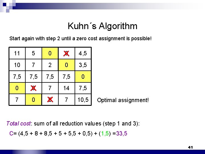
Kuhn´s Algorithm Start again with step 2 until a zero cost assignment is possible! 11 5 0 0 4, 5 10 7 2 0 3, 5 7, 5 0 0 0 7 14 7, 5 7 0 0 7 10, 5 Optimal assignment! Total cost: sum of all reduction values (step 1 and 3): C= (4, 5 + 8, 5 + 5, 5 + 0, 5) + (1, 5) =33, 5 41

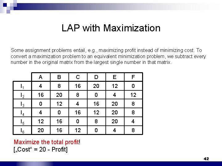
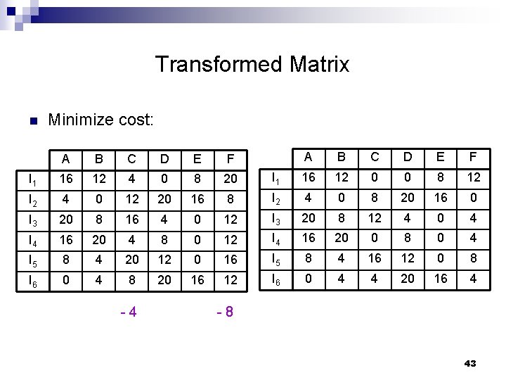
LAP with Maximization Some assignment problems entail, e. g. , maximizing profit instead of minimizing cost. To convert a maximization problem to an equivalent minimization problem, we subtract every number in the original matrix from the largest single number in that matrix. A B C D E F I 1 4 8 16 20 12 0 I 2 16 20 8 0 4 12 I 3 0 12 4 16 20 8 I 4 4 0 16 12 20 8 I 5 12 16 0 8 20 4 I 6 20 16 12 0 4 8 Maximize the total profit! [„Cost“ = 20 - Profit] 42

Transformed Matrix n Minimize cost: A B C D E F I 1 16 12 0 0 8 12 8 I 2 4 0 8 20 16 0 0 12 I 3 20 8 12 4 0 4 8 0 12 I 4 16 20 0 8 0 4 20 12 0 16 I 5 8 4 16 12 0 8 8 20 16 12 I 6 0 4 4 20 16 4 A B C D E F I 1 16 12 4 0 8 20 I 2 4 0 12 20 16 I 3 20 8 16 4 I 4 16 20 4 I 5 8 4 I 6 0 4 - 8 43

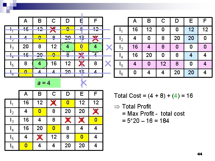
A B C D E F I 1 16 12 0 0 8 12 I 2 4 0 8 20 16 I 3 20 8 12 4 I 4 16 20 0 I 5 8 4 I 6 0 4 A B C D E F I 1 16 12 0 0 12 12 0 I 2 4 0 8 20 20 0 0 4 I 3 16 4 8 0 0 0 8 0 4 I 4 16 20 0 8 4 4 16 12 0 8 I 5 4 0 12 8 0 4 4 20 16 4 I 6 0 4 4 20 20 4 a = 4 A B C D E F I 1 16 12 0 0 12 12 I 2 4 0 8 20 20 0 I 3 16 4 8 0 0 0 I 4 16 20 0 8 4 4 I 5 4 0 12 8 0 4 I 6 0 4 4 20 20 4 Total Cost = (4 + 8) + (4) = 16 Total Profit = Max Profit - total cost = 5*20 – 16 = 184 44