OSSE Observation Simulation and Experiment Verification Developments q

OSSE Observation Simulation and Experiment Verification Developments q New simulation of run history PREPQC files with QC information q Simulation of SBUV BUFR ozone observations q Create simulated BUFR AMSUa, AMSUb, and GOES files (w/Tong Zhu) q Updated version of DBL 91 files produced with GSI h/v thinning info q Optimized experiment cycle script provides 15: 1 production speedup q Suru fit files/plots adapted for OSSE calibration experiments q Scatter fit plots developed for experiment comparisons q Radiance fit plots to examine results of bias correction experiments

Simulated SBUV Ozone Retrievals Simulating the SBUV retrievals involves converting the 91 level ozone concentrations from the nature run into 12 layers of ozone amounts (DU). The plot checks the conversion by comparing the NR total ozone values with the total profile ozone derived by summing the simulated layer values.

Comparing simulated thinned files to real thinned files at the Nature Run beginning

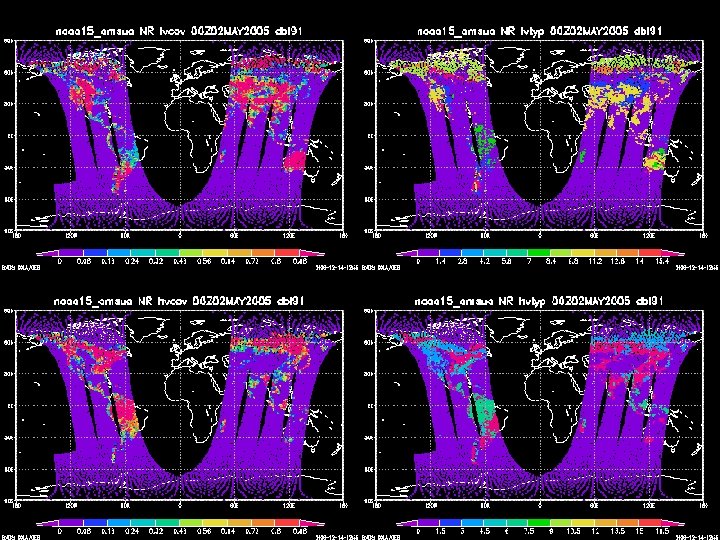
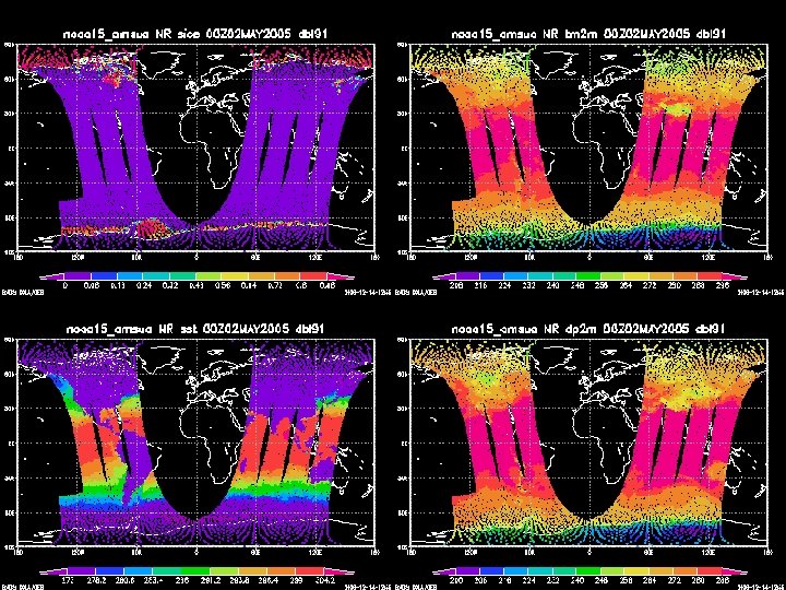
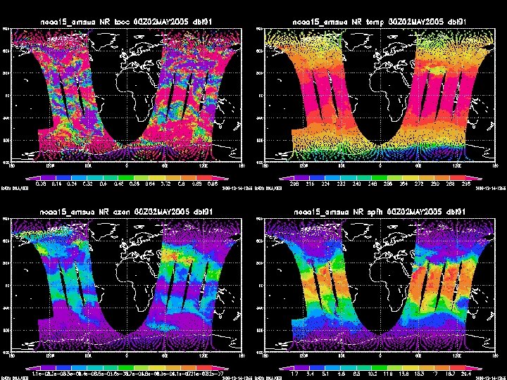
DBL 91 file structure – information for simulating radstat satellites NATURE RUN RADSTAT Binary file Sat location and geometry Surface type/veg from NCEP Surface quantities from NR 91 level upper air from NR BUFR Thinned BUFR file Complete BUFR report pointed to in RADSTAT file QC info for each channel

Contents of DBL 91 binary file From BUFR satellite file 2005. 00 1. 00 21. 00 3. 00 168. 67 59. 77 206. 00 570. 00 2. 00 1. 00 52. 79 59. 83. 00 813000. 00 004001 004002 004003 004004 004005 004006 006002 005002 001007 002019 005043 008012 007024 007025 010001 007002 YEAR MNTH DAYS HOUR MINU SECO CLON CLAT SAID SIID FOVN LSQL SAZA SOZA HOLS HMSL YEAR MONTH DAY HOUR MINUTE SECOND DEGREES CODE TABLE NUMERIC CODE TABLE DEGREE METER YEAR MONTH DAY HOUR MINUTE SECOND LONGITUDE LATITUDE SAT IDENTIFIER SAT INSTRUMENTS BEAM POSITION LAND/SEA QUALIFIER SAT ZENITH ANGLE SOLAR ZENITH ANGLE HEIGHT OF LAND SURFACE HEIGHT OR ALTITUDE From NCEP Climatology. 00000 iv=27 iv=28 iv=29 iv=30 ! ! low high vegetation cover type Surface quantities from Nature Run 31 32 33 34 44 45 50 57 58 59 78 79 129 136 137 1 2 3 4 5 6 7 8 9 10 11 12 13 14 15 Sea-ice cover [(0 -1)] Snow albedo [(0 -1)] Snow density [kg m**-3] Sea surface temperature [K] Snow evaporation [m of water] Snowmelt [m of water] Large-scale precipitation fraction [s] Downward uv radiation at the surface [w m**-2 s] Photosynthetically active radiation [w m**-2 s] Convective available potential energy [J kg**-1] Total column liquid water [kg m**-2] Total column ice water [kg m**-2] Geopotential [m**2 s**-2] Total column water [kg m**-2] Total column water vapour [kg m**-2] 141 142 143 144 145 146 147 148 151 152 159 164 165 166 167 168 169 172 175 176 177 178 179 180 181 182 186 187 188 189 195 196 197 198 205 206 208 209 210 211 235 238 243 244 245 16 17 18 19 20 21 22 23 24 25 26 27 28 29 30 31 32 33 34 35 36 37 38 39 40 41 42 43 44 45 46 47 48 49 50 51 52 53 54 55 56 57 58 59 60 Snow depth [m of water equivalent] Stratiform precipitation [m] Convective precipitation [m] Snowfall (convective + stratiform) [m of water equ Boundary layer dissipation [W m**-2 s] Surface sensible heat flux [W m**-2 s] Surface latent heat flux [W m**-2 s] Charnock Mean sea-level pressure [Pa] Surface pressure {pa] Boundary layer height [m] Total cloud cover [(0 - 1)] 10 metre U wind component [m s**-1] 10 metre V wind component [m s**-1] 2 metre temperature [K] 2 metre dewpoint temperature [K] Surface solar radiation downwards [W m**-2 s] Land/sea mask [(0, 1)] Surface thermal radiation downwards [W m**-2 s] Surface solar radiation [W m**-2 s] Surface thermal radiation [W m**-2 s] Top solar radiation [W m**-2 s] Top thermal radiation [W m**-2 s] East/West surface stress [N m**-2 s] North/South surface stress [N m**-2 s] Evaporation [m of water] Low cloud cover [(0 - 1)] Medium cloud cover [(0 - 1)] High cloud cover [(0 - 1)] Sunshine duration [s] Lat. component of gravity wave stress [N m**-2 s] Meridional component of gravity wave stress [N m** Gravity wave dissipation [W m**-2 s] Skin reservoir content [m of water] Runoff [m] Total column ozone [Dobson] Top net solar radiation, clear sky [W m**-2] Top net thermal radiation, clear sky [W m**-2] Surface net solar radiation, clear sky [W m**-2] Surface net thermal radiation, clear sky [W m**-2] Skin temperature [K] Temperature of snow layer [K] Forecast albedo [(0 - 1)] Forecast surface roughness [m] Forecast log of surface roughness for heat NR 91 levels of: pres cloudcov cloudice cloudh 2 o ozone mmr temperature spfhumid

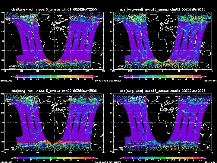
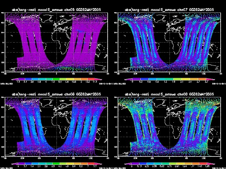
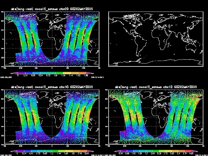
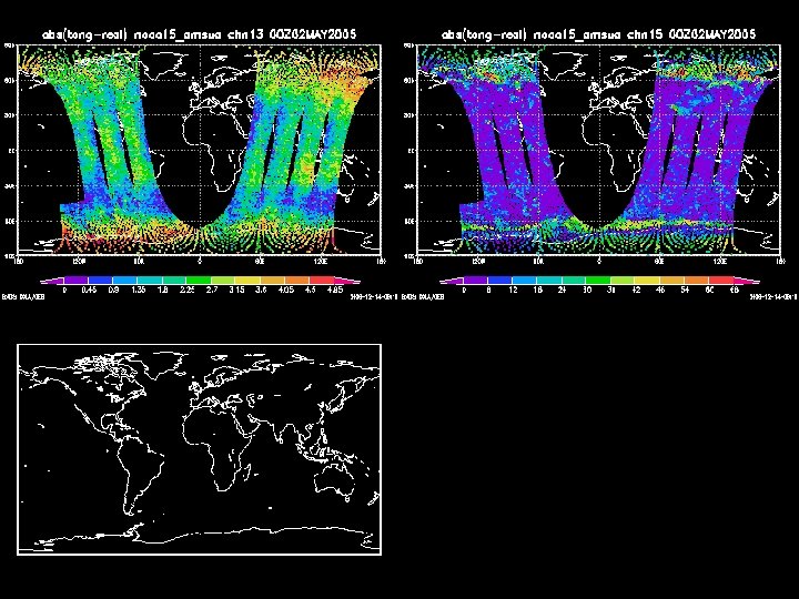
Some Examples of DBL 91 binary file contents

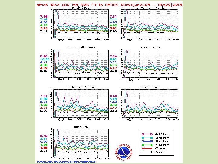
Fit files storage and display “Suru” fit files contain rms, means, and counts of ob-bg Seven regions: GL, NH, SH, TR, NA, EU, AS RAOB SURF ACFT ACAR ps, 21 levels of q, t, u, v, z, 7 regions ps from adpsfc and sfcshp, 7 regions t, z, u, v, spd, 1000 -700, 700 -300, 300 -150, NA only Filenames have the form fnn. type. date, ie f 00. raob. 2005070100 Each file has fits for 1 lead time, 1 datatype, 7 regions, 1 valid time GRADS combines these files to produce time series or scatter fit plots Suru plots create f 00, f 06, f 12, f 24, f 36, f 48 for raob surf acft acar. 5 MB contains the complete set of Suru fit files for 1 year

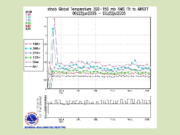
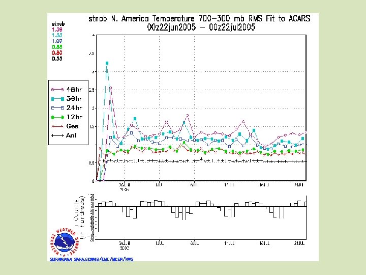
Examples of Suru Time Series Fits

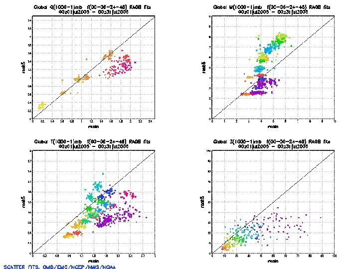
Scatter Fit Comparison Plots Need to compare two experiments – use scatter plot Compare all levels and forecast lengths for each variable Comparison with real data case is relevant for calibration Forecast lengths out to 5 days or more can be added Develop a simple way to denote levels and forecast length

Analysis and Forecast fit scatter plot comparison with realn Fits between each calibration run are compared with the realn case on a scatter plot. Each dot compares two global average RMS fits for 1 variable, 1 forecast length, one level, and one synoptic time. Dots are plotted for every case where the realn run coincides in space/time with a calibration run. Pressure levels indicated by dot colors 200 green 250 yellow/green 300 yellow 500 dark yellow 700 orange 850 red 1000 magenta 10 20 30 50 70 100 150 purple dark blue medium blue light blue aqua Forecast length indicated by dot size - longer length - bigger dot

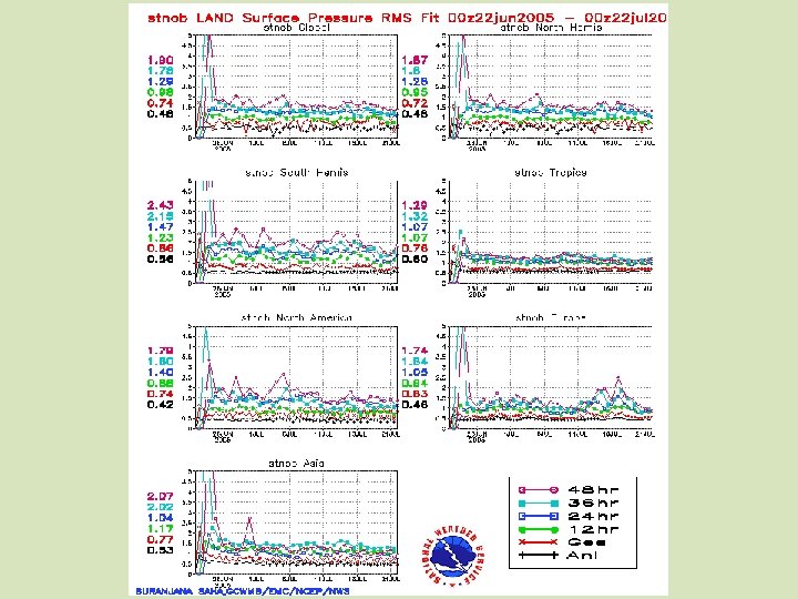
Summary of Calibration Experiments realn - real data run, 3 jul-15 jul perfn - perfect data run, 22 jun-15 jul cnverr - simulated data with small errors, 1 jul-18 jul raob 5 - simulated data with bigger raob errors, 1 jul-18 jul stnob - like cnverr w/sat bias correction initially zero, 22 jun-22 jul gsitest - like raob 5 with modified GSI error specs, 1 jul-18 jul synth - simulated perfect data but w/o radiosondes, 3 jul-15 jul synt 2 - simulated perfect data, 3 jul-15 jul

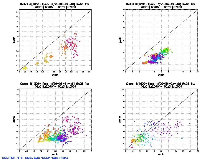
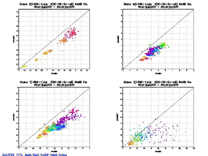
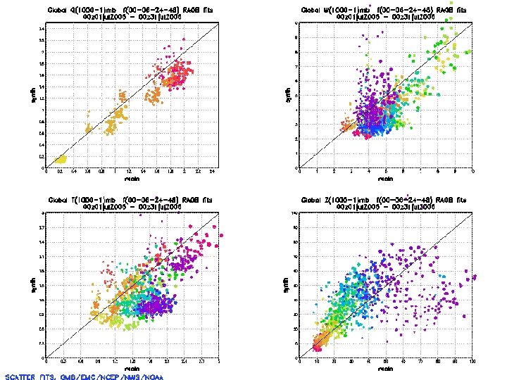
This plot is interesting because it shows perfect data w/o raobs performs about the same as real data including raobs, at least by this measure

Radiance Time Series Fit Plots A question arose concerning application of the bias correction to simulated radiance data Nikki and Yuanfu made some runs to examine several scenarios: 1) Operational bias correction coefficients used 2) Bias correction with coefficients initialized to zero 3) No bias correction (turned off) After running the experiments, time series traces of the ob-fg global RMS and mean values were plotted for each satellite instrument and channel. Many of the cases were insensitive to whether or what kind of bias correction was applied. A number of cases however showed distinct differences between the various approaches. A representative sample of those cases follow, with some analysis given. Each line in the following plots is color coded to represent the experiment whose description is the same color in the legend above.

Needs bias correction

Operational coefs spin down close to zero

Here bias correction doesn’t help

Operational bias correction coefs start off and stay off

Bias corrections way off No bias correction is better

Operational bc coefs are slow to respond; large difference in accepted data

Interesting difference in accepted data counts considering how close to zero are the fits are