Organizing Data Proportions Percentages Rates and rates of

Organizing Data Proportions, Percentages, Rates, and rates of change.

Raw Data n n n Often hard to interpret just a bunch of raw scores Raw scores can be transformed to show patterns and trends in the data Most useful is the frequency distribution or table

Frequency Tables will have: n n Informative title Two columns for nominal data: (1) response and (2) frequency (How often did certain responses occur? )

Standardizing data Proportion: compare the number of cases for each response (frequency, f) with the total number of cases (N). Proportion = frequency / number = f / N n In the previous example, 20 out of 45 students earned a B, so the proportion earning a B is 20/45 =. 4444, which (rounding to 2 decimals more than the original data) =. 44 n

n n n Percentage is the frequency per 100 cases. (It is a special case of a proportion. ) Percentage = 100 (f / N) People are “used” to thinking in percentages (such as in cents per dollar. . ).

Example n n 20 our of 45 students earned a B in a course. Proportion = f / N = 20/45 = 0. 44 Percentage = 100 (20/35) = 44% (Per cent means per 100, and we write it 0/0. Per thousand would be 0/00)

Ratios n n A ratio of “a” to “b” is the frequency of “a” compared to the frequency of “b”, with the frequency of “a” coming first, or in the numerator, just as it does in the sentence. a/b or sometimes expressed as a: b

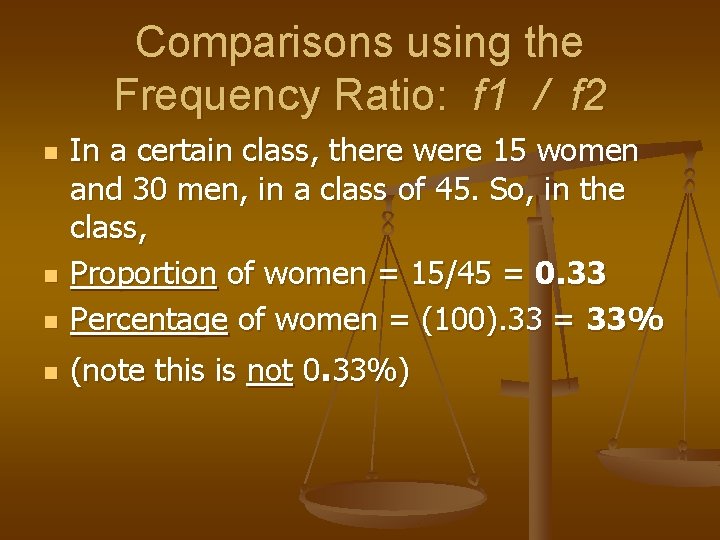
Comparisons using the Frequency Ratio: f 1 / f 2 n In a certain class, there were 15 women and 30 men, in a class of 45. So, in the class, Proportion of women = 15/45 = 0. 33 Percentage of women = (100). 33 = 33% n (note this is not 0. 33%) n n

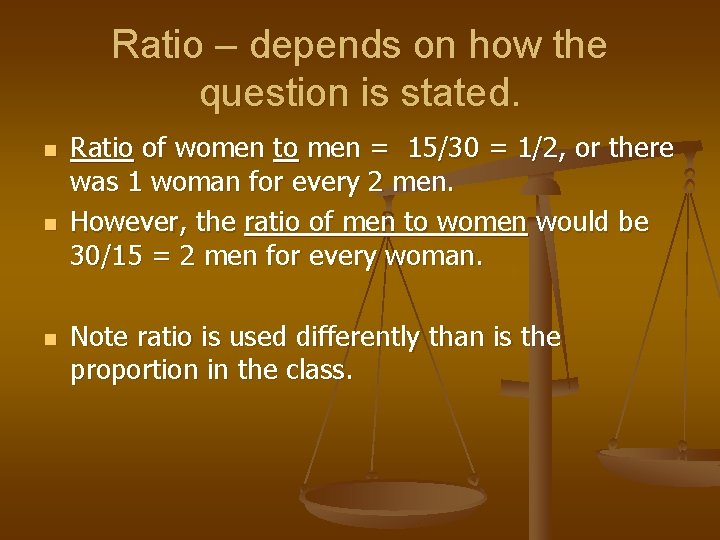
Ratio – depends on how the question is stated. n n n Ratio of women to men = 15/30 = 1/2, or there was 1 woman for every 2 men. However, the ratio of men to women would be 30/15 = 2 men for every woman. Note ratio is used differently than is the proportion in the class.

Rate n n A rate indicates the number of actual cases compared to the number of potential cases. Pretty subtle, eh? For population studies, these are usually expressed as the number of actual cases per 1000 potential cases (usually per 1000 people in the population).

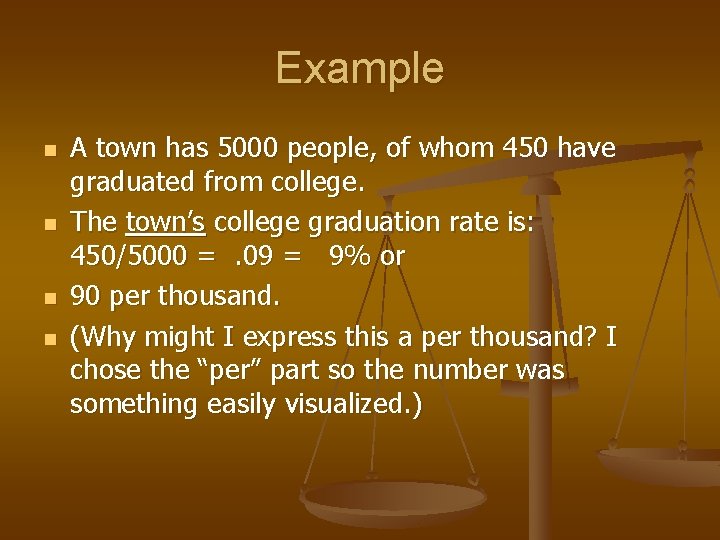
Example n n A town has 5000 people, of whom 450 have graduated from college. The town’s college graduation rate is: 450/5000 =. 09 = 9% or 90 per thousand. (Why might I express this a per thousand? I chose the “per” part so the number was something easily visualized. )

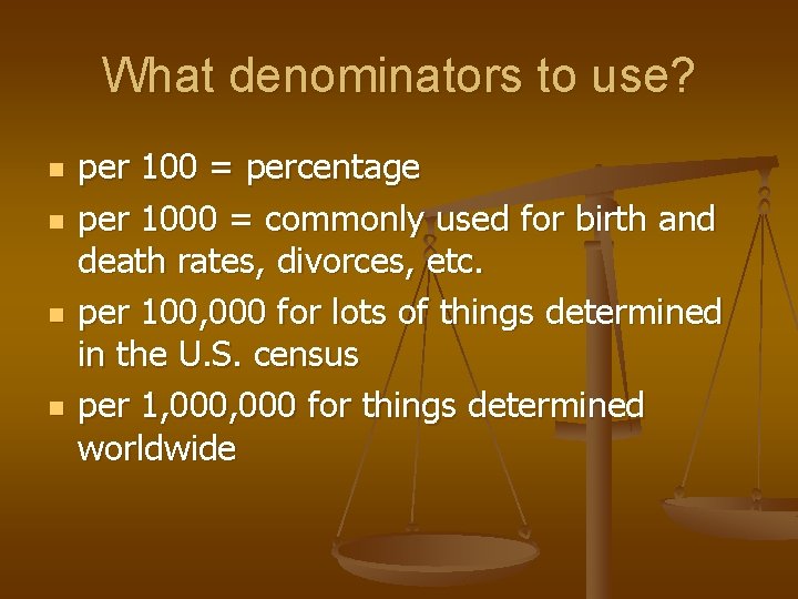
What denominators to use? n n per 100 = percentage per 1000 = commonly used for birth and death rates, divorces, etc. per 100, 000 for lots of things determined in the U. S. census per 1, 000 for things determined worldwide

Generalization n n Use the denominator that gives you the simplest whole number, easiest for you to grasp. Usually this is a number between 1 and 100. It’s hard for people to visualize the meaning of very small or large numbers such as 0. 00123, or 132, 431, 000

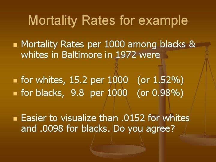
Mortality Rates for example n n Mortality Rates per 1000 among blacks & whites in Baltimore in 1972 were for whites, 15. 2 per 1000 (or 1. 52%) for blacks, 9. 8 per 1000 (or 0. 98%) Easier to visualize than. 0152 for whites and. 0098 for blacks. Do you agree?

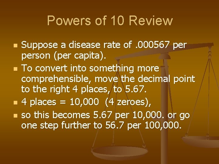
Powers of 10 Review n n Suppose a disease rate of. 000567 person (per capita). To convert into something more comprehensible, move the decimal point to the right 4 places, to 5. 67. 4 places = 10, 000 (4 zeroes), so this becomes 5. 67 per 10, 000. or go one step further to 56. 7 per 100, 000.

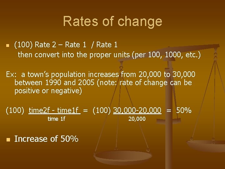
Rates of change n (100) Rate 2 – Rate 1 / Rate 1 then convert into the proper units (per 100, 1000, etc. ) Ex: a town’s population increases from 20, 000 to 30, 000 between 1990 and 2005 (note: rate of change can be positive or negative) (100) time 2 f - time 1 f = (100) 30, 000 -20, 000 = 50% time 1 f n Increase of 50% 20, 000

“Organizing the Data” Review of: Frequency Distributions & Histograms

Frequency Distributions n List or plot data n Nominal Data -- in any order n Ordinal & Interval Data – Usually highest number at top of table to lowest number at bottom of the table

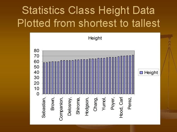
Statistics Class Height Data Plotted from shortest to tallest

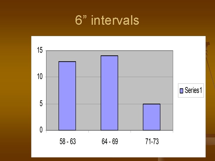
Intervals – Grouping Data n n n range of values in the data set numbers of class intervals desired size of class interval upper limit of a class interval lower limit of a class interval

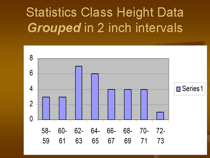
Statistics Class Height Data Grouped in 2 inch intervals

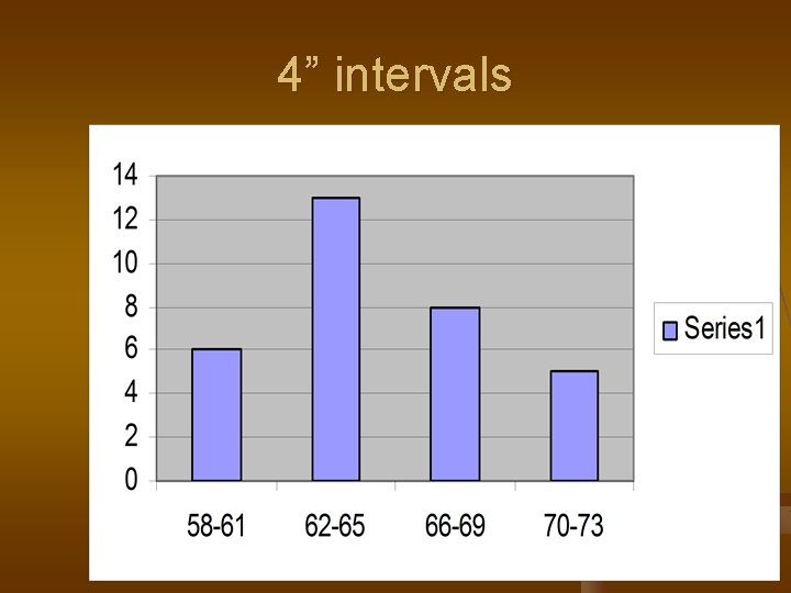
4” intervals

6” intervals

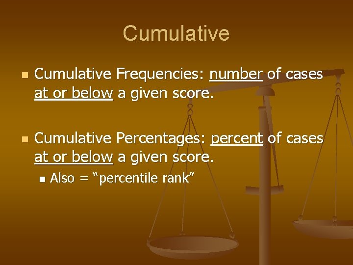
Cumulative n n Cumulative Frequencies: number of cases at or below a given score. Cumulative Percentages: percent of cases at or below a given score. n Also = “percentile rank”

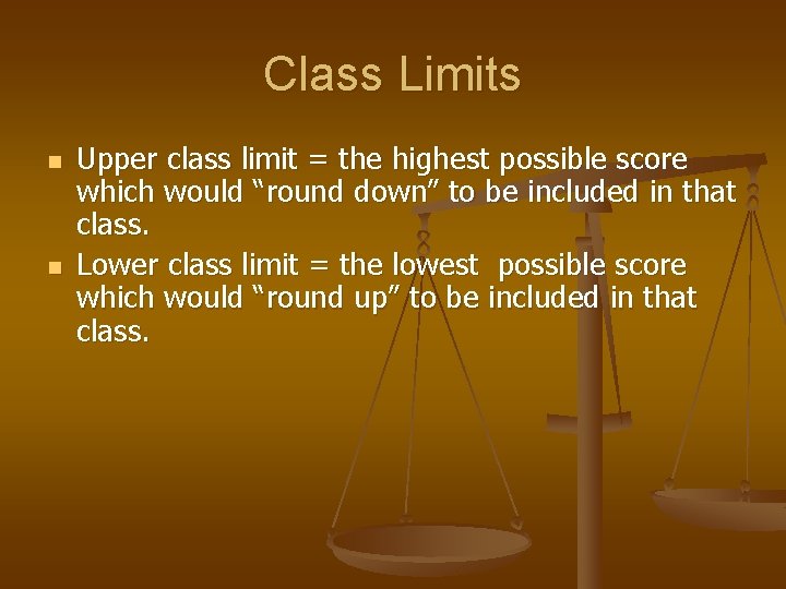
Class Limits n n Upper class limit = the highest possible score which would “round down” to be included in that class. Lower class limit = the lowest possible score which would “round up” to be included in that class.

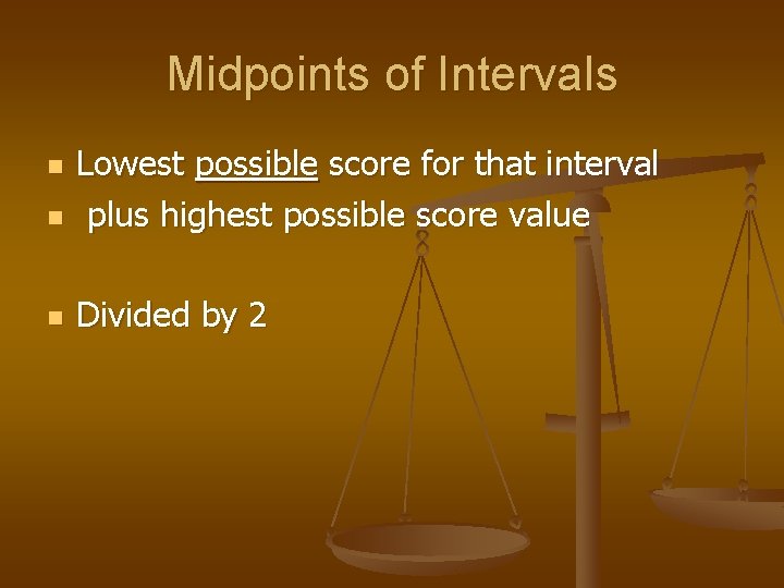
Midpoints of Intervals n Lowest possible score for that interval plus highest possible score value n Divided by 2 n

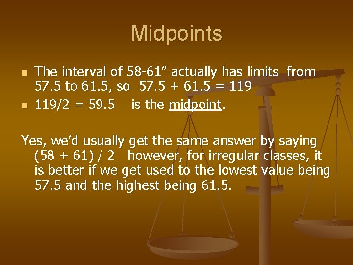
Midpoints n n The interval of 58 -61” actually has limits from 57. 5 to 61. 5, so 57. 5 + 61. 5 = 119/2 = 59. 5 is the midpoint. Yes, we’d usually get the same answer by saying (58 + 61) / 2 however, for irregular classes, it is better if we get used to the lowest value being 57. 5 and the highest being 61. 5.

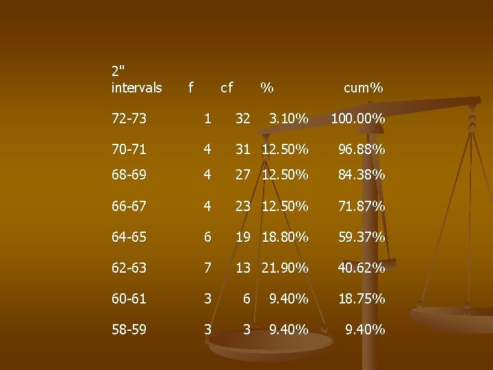
Cumulative Frequency n n To expand our frequency table, add columns for cumulative frequency, percent, and cumulative percent. Arrange your scores from low at the bottom to high at the top. Then, the Cumulative Frequency is simply the frequency of scores at or below the value in question.

Percentile Rank n = the cumulative percentage n n n The % at or below that score So for a height of 5’ 4”, or 64”, what is the percentile rank in our height data? The following chart shows frequency, cum. freq. , percentage, & cumulative %.

2" intervals f cf % cum% 72 -73 1 32 3. 10% 100. 00% 70 -71 4 31 12. 50% 96. 88% 68 -69 4 27 12. 50% 84. 38% 66 -67 4 23 12. 50% 71. 87% 64 -65 6 19 18. 80% 59. 37% 62 -63 7 13 21. 90% 40. 62% 60 -61 3 6 9. 40% 18. 75% 58 -59 3 3 9. 40%

Percentile Rank n n n 64 -65” has a cumulative percent of 59. 37%, so 59. 37% of class is in this category or shorter than this category. 62 -63 “ has a cumulative percent of 40. 62%, so 40. 62% of class is in this category or shorter than this category So, percentile rank = cumulative percent when looking at the raw data -- but it is more complex for grouped data, so be wary.

Cross-tabulations

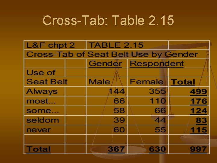
Cross-Tabulation: n n Cross-tabulation review: a table which presents the distribution of one variable (frequency and/or %) across the categories of one or more additional variables.

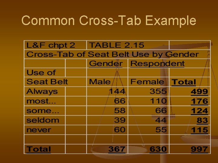
Common Cross-Tab Example

Cross-Tab: Table 2. 15 n n n If asking questions about the differences between males & females in seat belt use, use column percents. If asking questions about different uses of seat belts by the population as a whole, use the row percents. Hint: If totals are not given -- put them in before you start to evaluate.

Cross-Tab: Table 2. 15

Data Format on SPSS n Note that when you are working with raw data sets on the computer, you will put each case in a row, rather than making a cross-tabulation table. We will do this when we work with SPSS.