Ordinary Differential Equations JyunMing Chen 1 Contents Review

Ordinary Differential Equations Jyun-Ming Chen 1

Contents • Review • Euler’s method • 2 nd order methods – Midpoint – Heun’s • • Systems of ODE Stability Issue Implicit Methods Adaptive Stepsize • Runge-Kutta Method 2

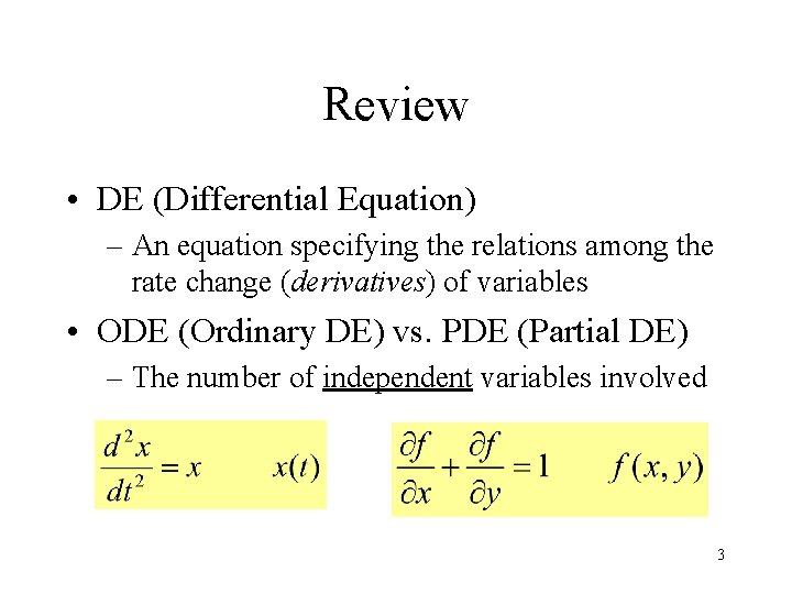
Review • DE (Differential Equation) – An equation specifying the relations among the rate change (derivatives) of variables • ODE (Ordinary DE) vs. PDE (Partial DE) – The number of independent variables involved 3

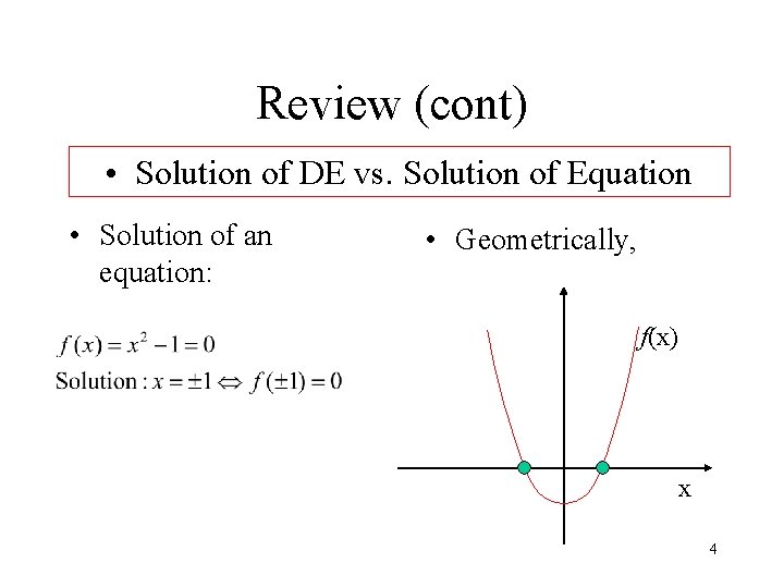
Review (cont) • Solution of DE vs. Solution of Equation • Solution of an equation: • Geometrically, f(x) x 4

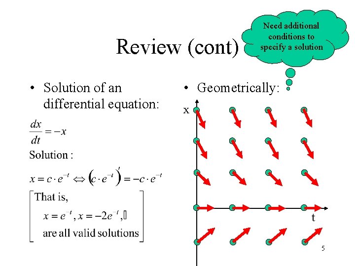
Review (cont) • Solution of an differential equation: Need additional conditions to specify a solution • Geometrically: x t 5

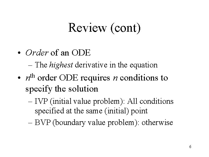
Review (cont) • Order of an ODE – The highest derivative in the equation • nth order ODE requires n conditions to specify the solution – IVP (initial value problem): All conditions specified at the same (initial) point – BVP (boundary value problem): otherwise 6

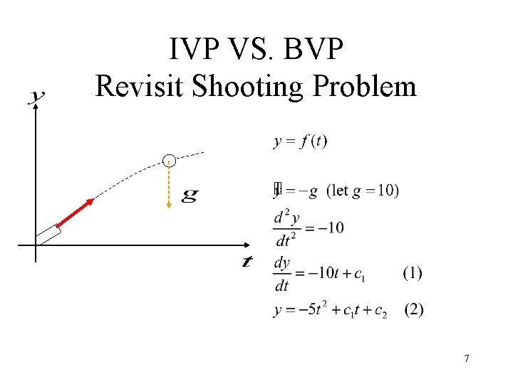
IVP VS. BVP Revisit Shooting Problem 7

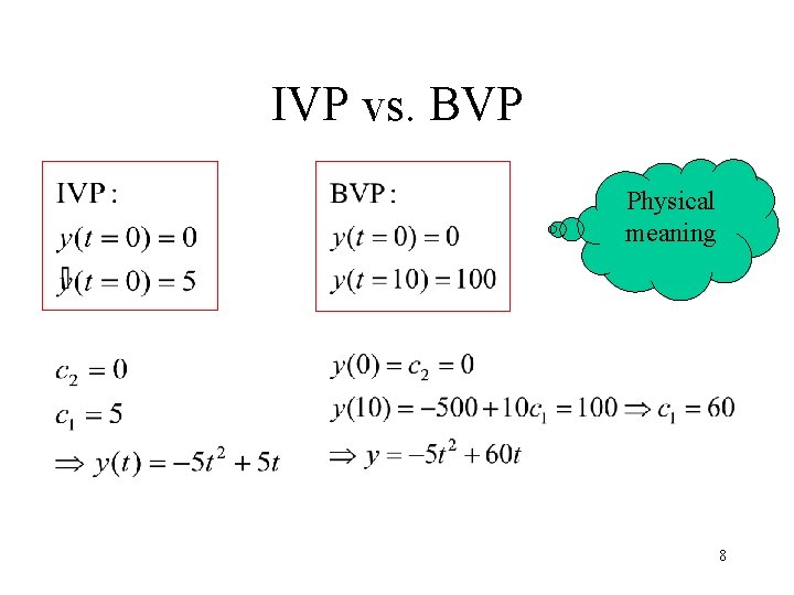
IVP vs. BVP Physical meaning 8

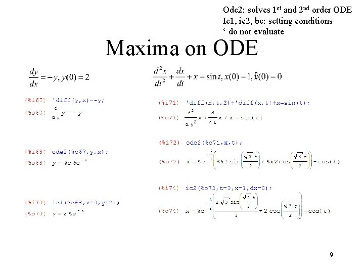
Ode 2: solves 1 st and 2 nd order ODE Ic 1, ic 2, bc: setting conditions ‘ do not evaluate Maxima on ODE 9

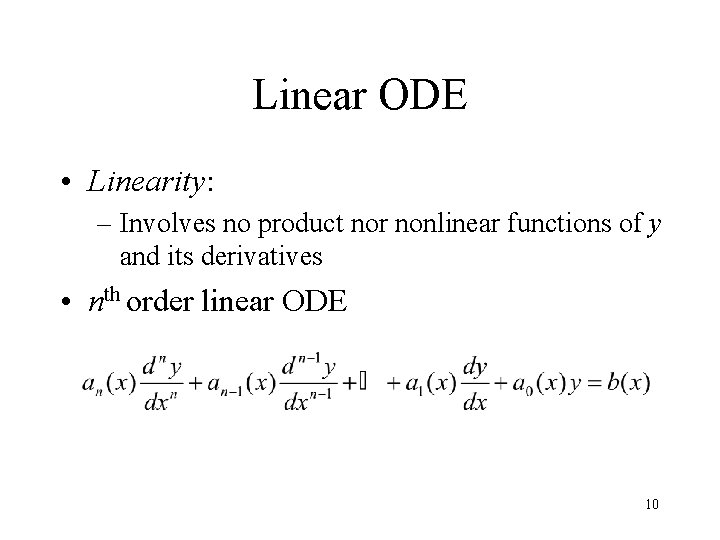
Linear ODE • Linearity: – Involves no product nor nonlinear functions of y and its derivatives • nth order linear ODE 10

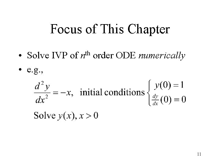
Focus of This Chapter • Solve IVP of nth order ODE numerically • e. g. , 11

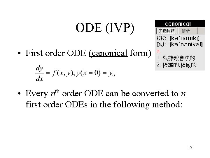
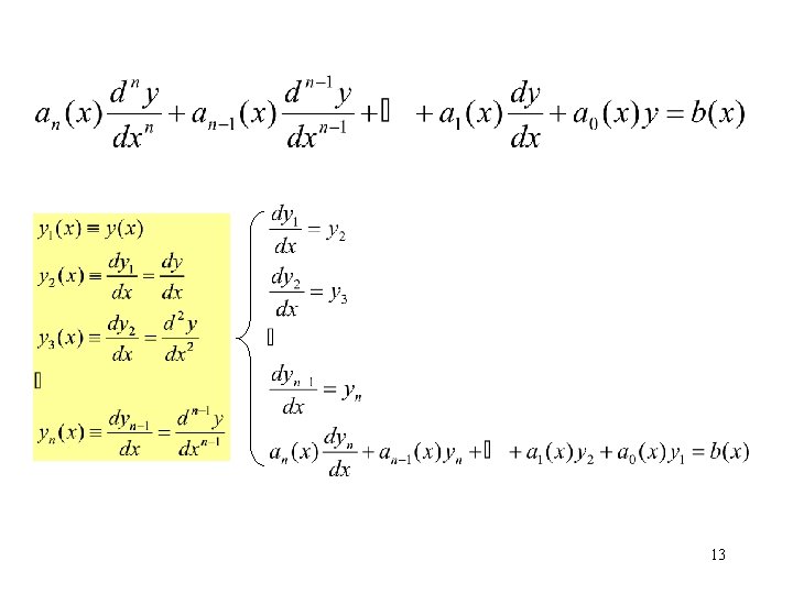
ODE (IVP) • First order ODE (canonical form) • Every nth order ODE can be converted to n first order ODEs in the following method: 12

13

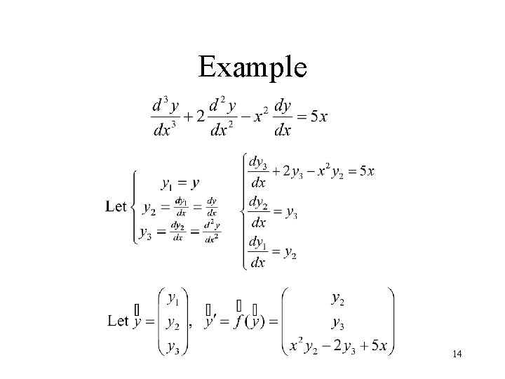
Example 14

End of Review 15

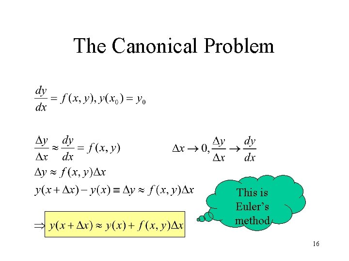
The Canonical Problem This is Euler’s method 16

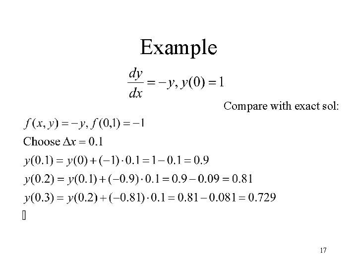
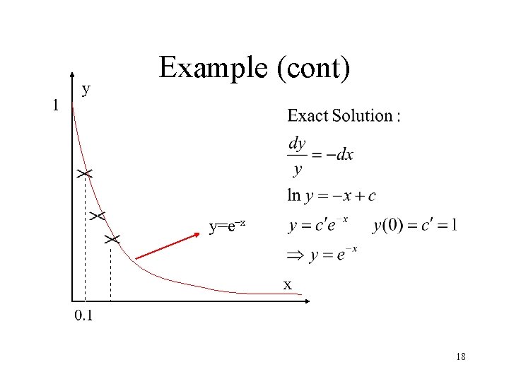
Example Compare with exact sol: 17

1 y Example (cont) y=e–x x 18

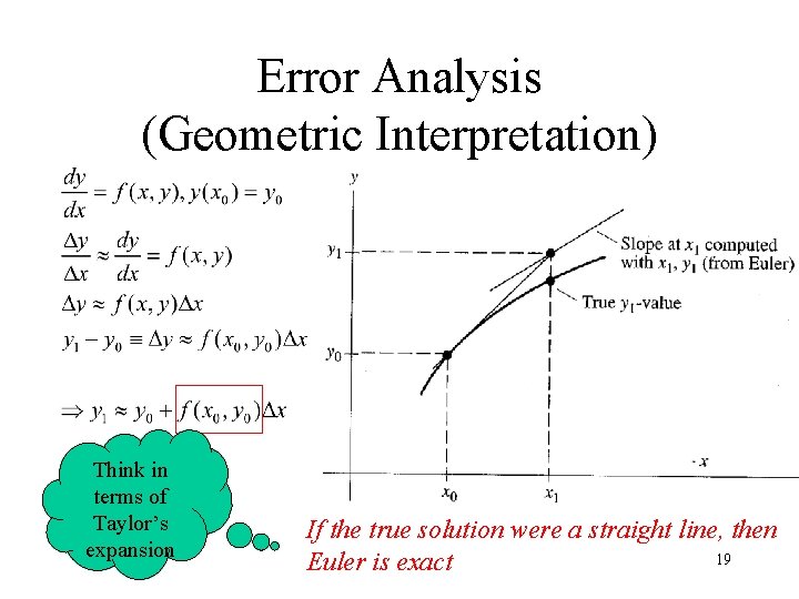
Error Analysis (Geometric Interpretation) Think in terms of Taylor’s expansion If the true solution were a straight line, then 19 Euler is exact

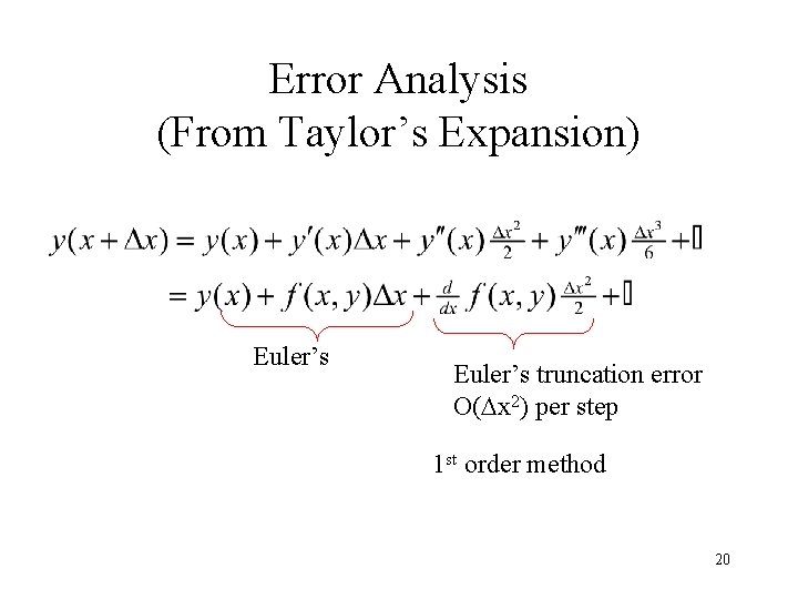
Error Analysis (From Taylor’s Expansion) Euler’s truncation error O(Dx 2) per step 1 st order method 20

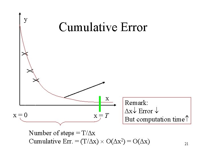
y Cumulative Error x x=0 x=T Remark: Dx Error But computation time Number of steps = T/Dx Cumulative Err. = (T/Dx) O(Dx 2) = O(Dx) 21

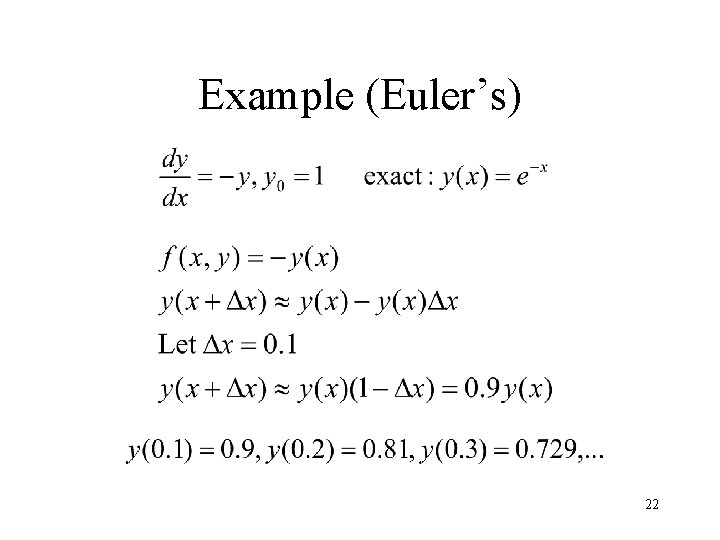
Example (Euler’s) 22

Methods Improving Euler Motivated by Geometric Interpretation 23

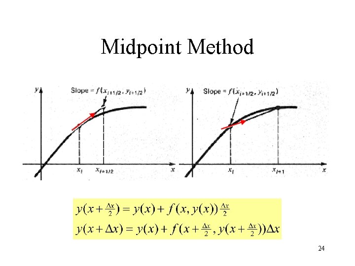
Midpoint Method 24

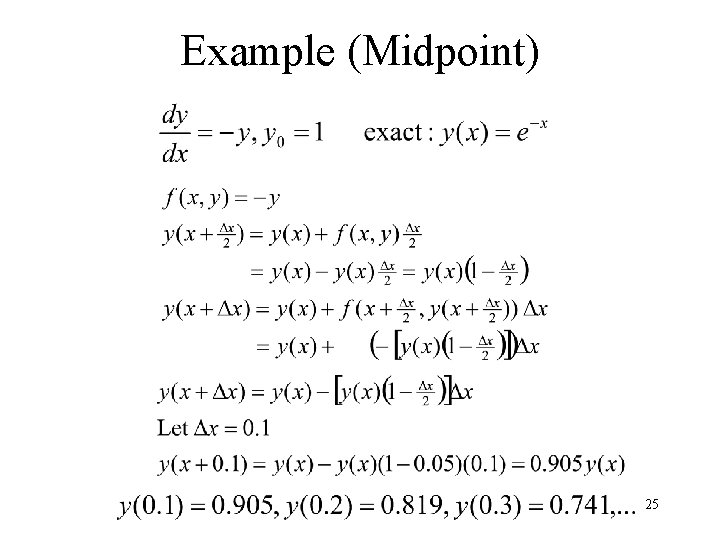
Example (Midpoint) 25

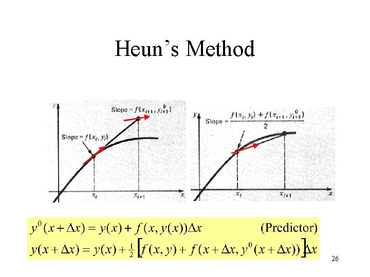
Heun’s Method 26

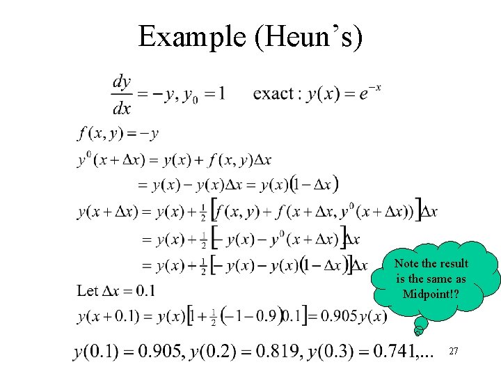
Example (Heun’s) Note the result is the same as Midpoint!? 27

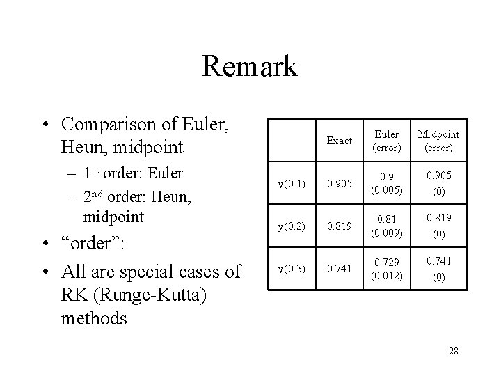
Remark • Comparison of Euler, Heun, midpoint – 1 st order: Euler – 2 nd order: Heun, midpoint • “order”: • All are special cases of RK (Runge-Kutta) methods Exact Euler (error) Midpoint (error) y(0. 1) 0. 905 0. 9 (0. 005) 0. 905 (0) y(0. 2) 0. 819 0. 81 (0. 009) 0. 819 (0) y(0. 3) 0. 741 0. 729 (0. 012) 0. 741 (0) 28

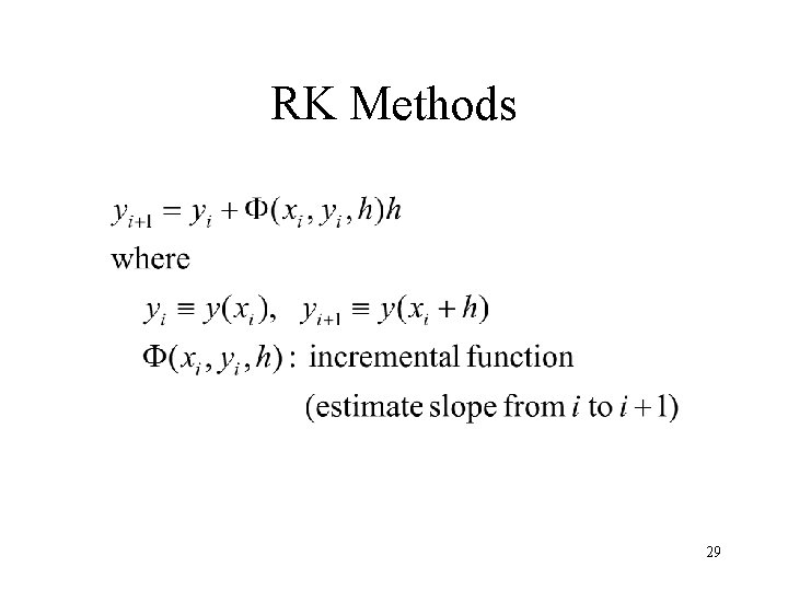
RK Methods 29

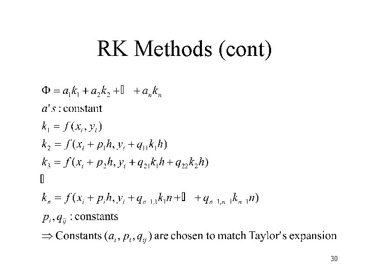
RK Methods (cont) 30

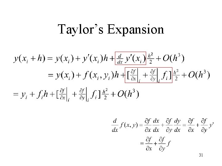
Taylor’s Expansion 31

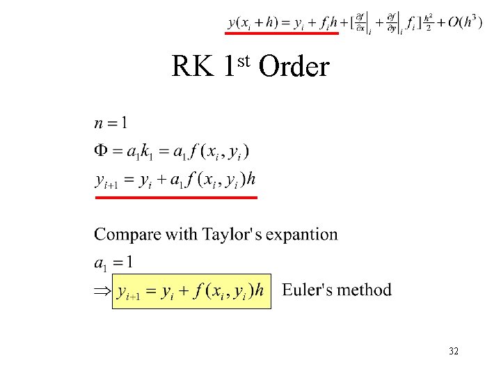
RK st 1 Order 32

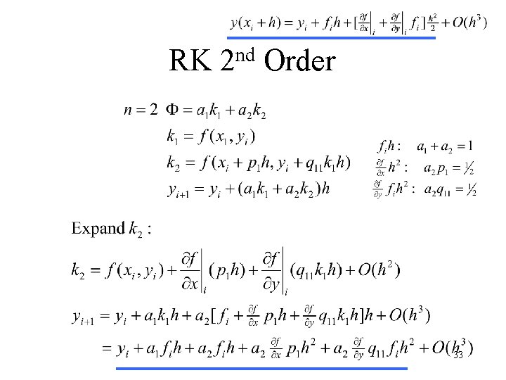
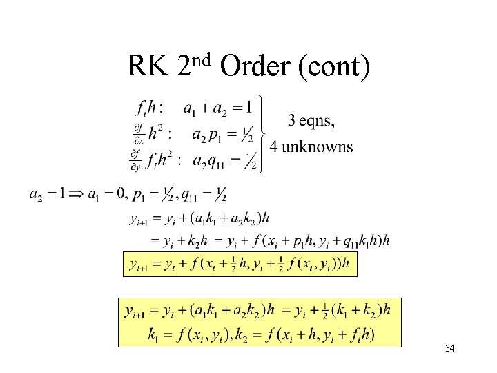
RK nd 2 Order 33

RK nd 2 Order (cont) 34

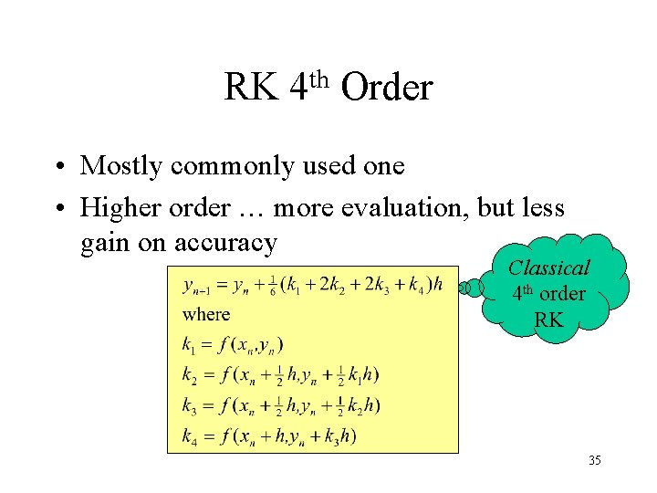
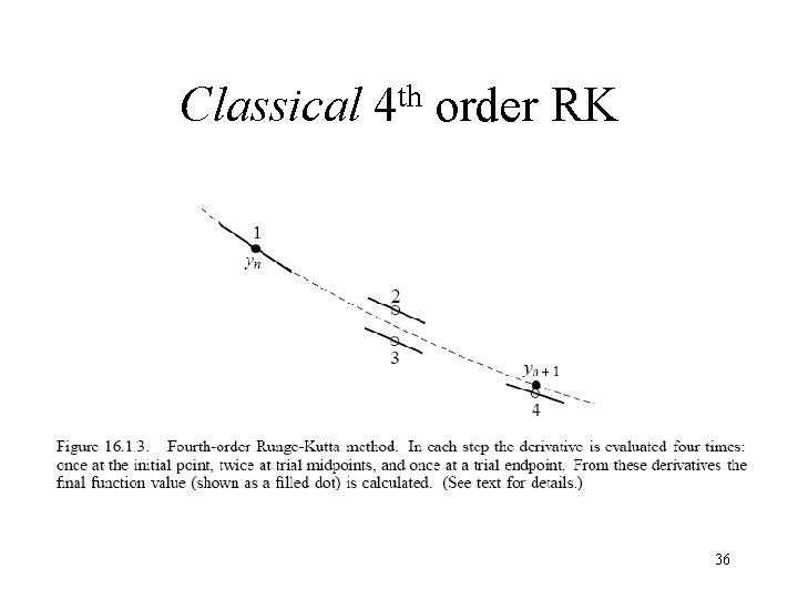
RK th 4 Order • Mostly commonly used one • Higher order … more evaluation, but less gain on accuracy Classical 4 th order RK 35

Classical th 4 order RK 36

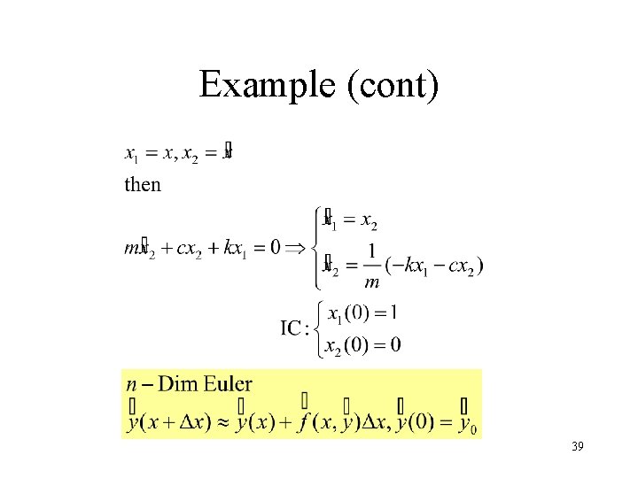
System of ODE • Convert higher order ODE to 1 st order ODEs • All methods equally apply, in vector form 37

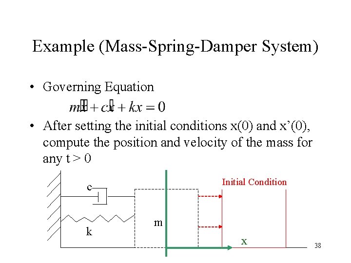
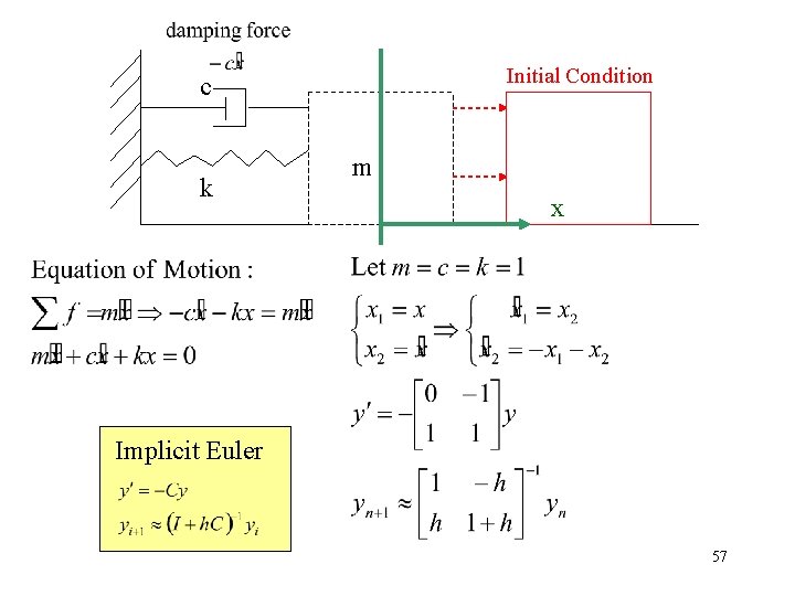
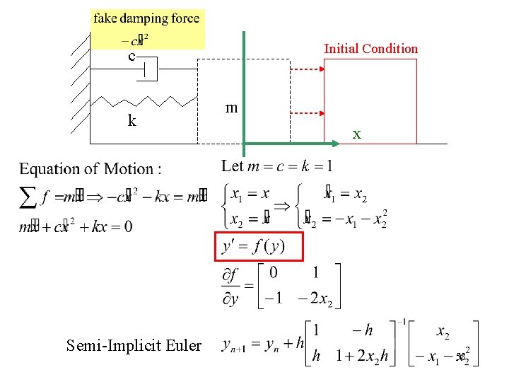
Example (Mass-Spring-Damper System) • Governing Equation • After setting the initial conditions x(0) and x’(0), compute the position and velocity of the mass for any t > 0 Initial Condition c k m x 38

Example (cont) 39

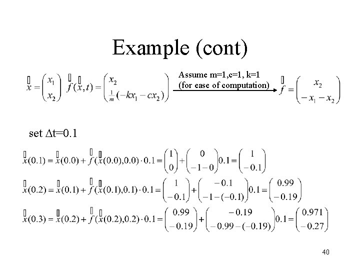
Example (cont) Assume m=1, c=1, k=1 (for ease of computation) set Dt=0. 1 40

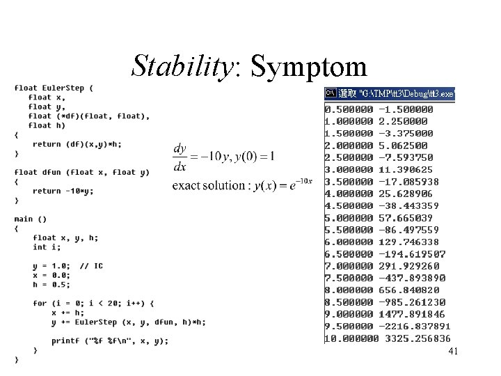
Stability: Symptom 41

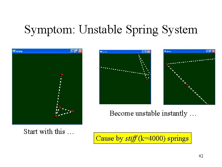
Symptom: Unstable Spring System Become unstable instantly … Start with this … Cause by stiff (k=4000) springs 42

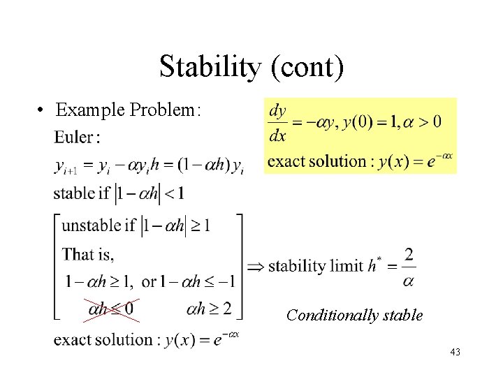
Stability (cont) • Example Problem: Conditionally stable 43

Discussion • Different algorithm different stability limit – Check Midpoint Method • Different problem different stability limit – use the previous problem as benchmark 44

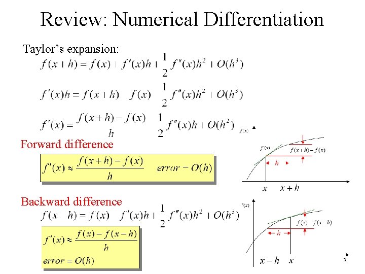
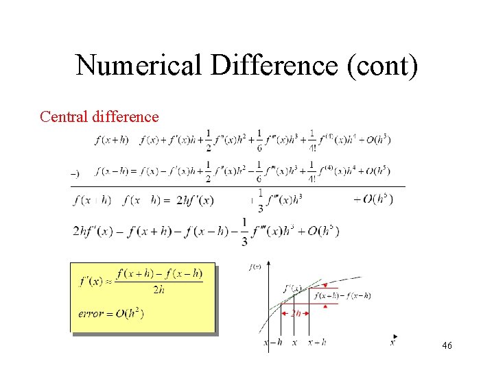
Review: Numerical Differentiation Taylor’s expansion: Forward difference Backward difference 45

Numerical Difference (cont) Central difference 46

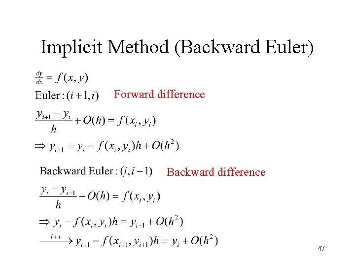
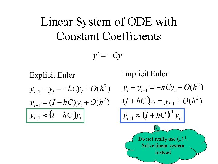
Implicit Method (Backward Euler) Forward difference Backward difference 47

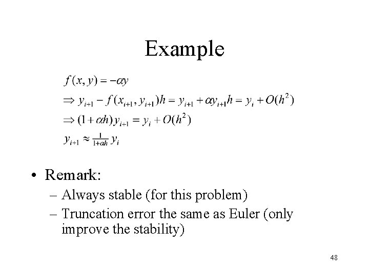
Example • Remark: – Always stable (for this problem) – Truncation error the same as Euler (only improve the stability) 48

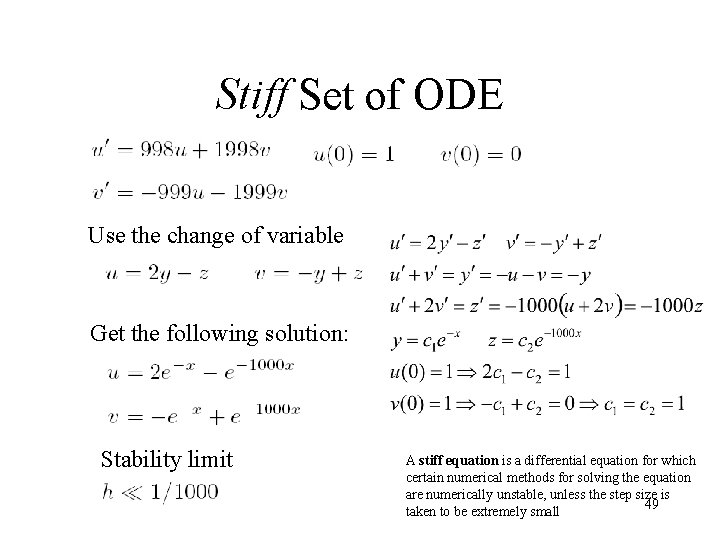
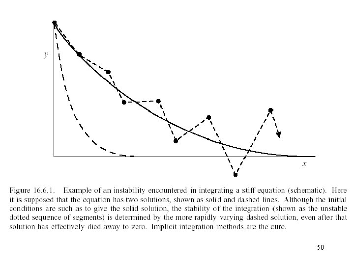
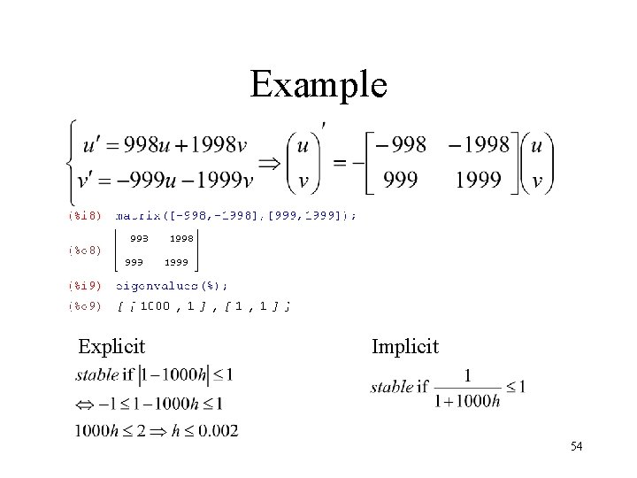
Stiff Set of ODE Use the change of variable Get the following solution: Stability limit A stiff equation is a differential equation for which certain numerical methods for solving the equation are numerically unstable, unless the step size is 49 taken to be extremely small

50

Linear System of ODE with Constant Coefficients Do not really use (. . )-1. Solve linear system instead 51

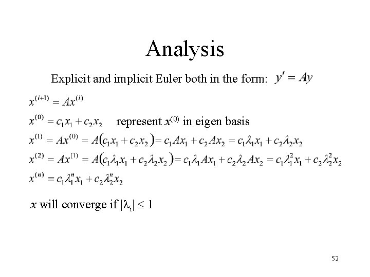
Analysis Explicit and implicit Euler both in the form: represent x(0) in eigen basis x will converge if |li| 1 52

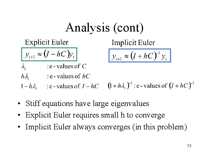
Analysis (cont) • Stiff equations have large eigenvalues • Explicit Euler requires small h to converge • Implicit Euler always converges (in this problem) 53

Example Explicit Implicit 54

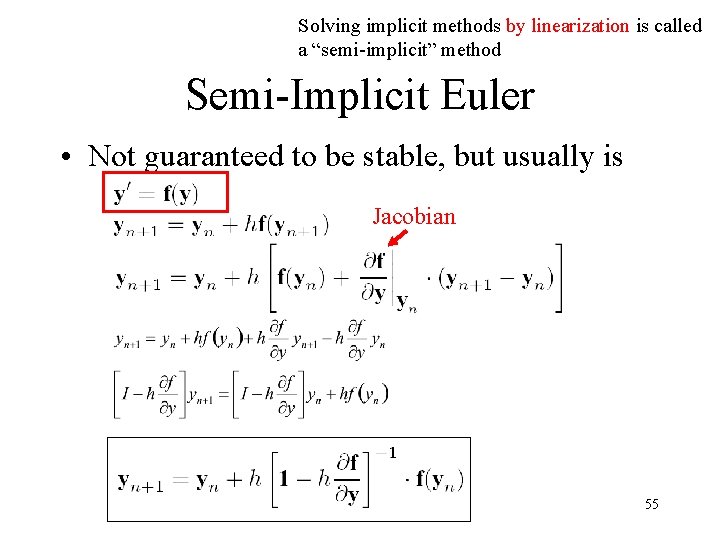
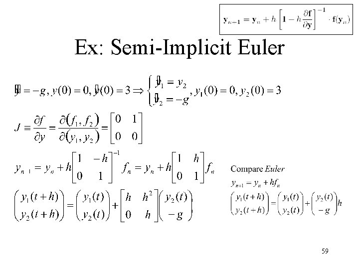
Solving implicit methods by linearization is called a “semi-implicit” method Semi-Implicit Euler • Not guaranteed to be stable, but usually is Jacobian 55

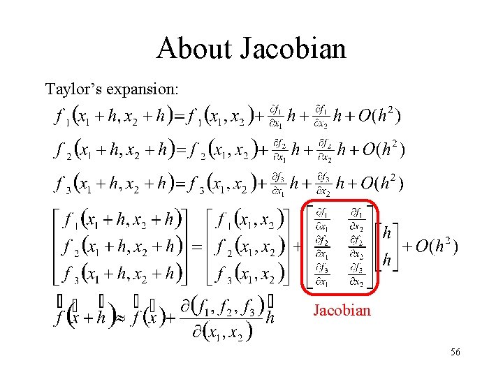
About Jacobian Taylor’s expansion: Jacobian 56

Initial Condition c k m x Implicit Euler 57

Initial Condition c k Semi-Implicit Euler m x 58

Ex: Semi-Implicit Euler 59

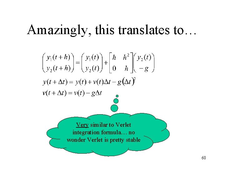
Amazingly, this translates to… Very similar to Verlet integration formula… no wonder Verlet is pretty stable 60

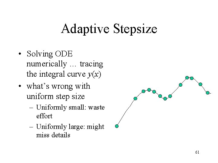
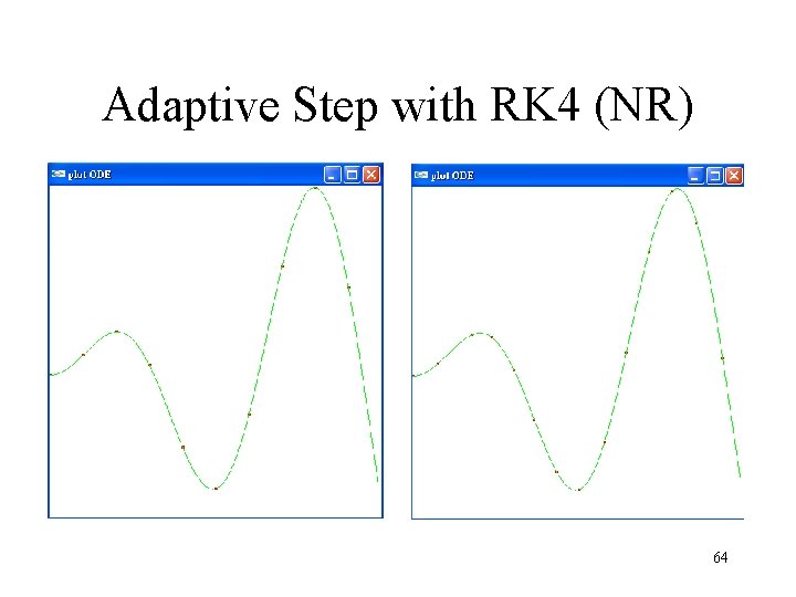
Adaptive Stepsize • Solving ODE numerically … tracing the integral curve y(x) • what’s wrong with uniform step size – Uniformly small: waste effort – Uniformly large: might miss details 61

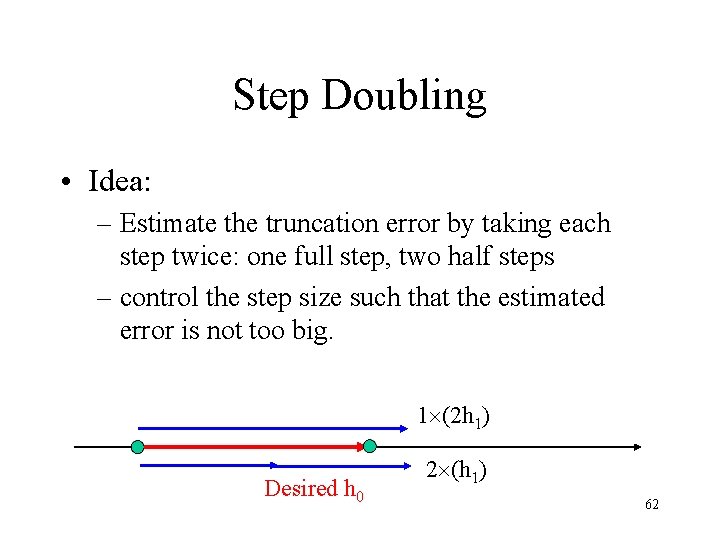
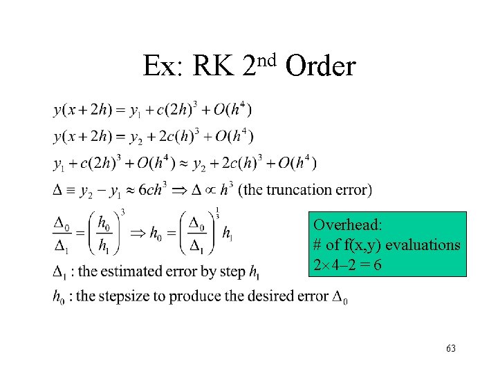
Step Doubling • Idea: – Estimate the truncation error by taking each step twice: one full step, two half steps – control the step size such that the estimated error is not too big. 1 (2 h 1) Desired h 0 2 (h 1) 62

Ex: RK nd 2 Order Overhead: # of f(x, y) evaluations 2 4– 2 = 6 63

Adaptive Step with RK 4 (NR) 64

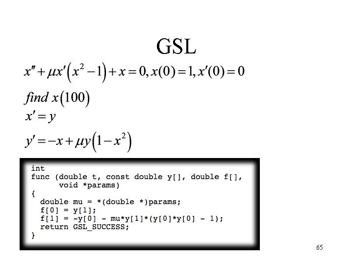
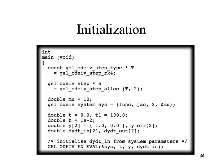
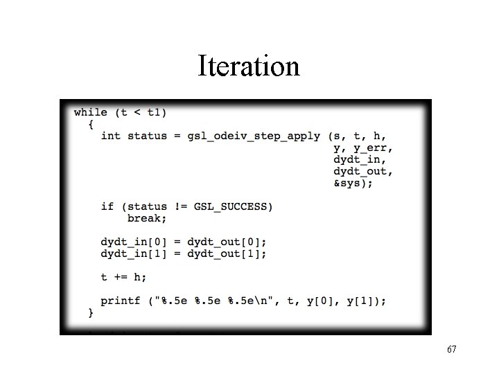
GSL 65

Initialization 66

Iteration 67