Ordinary Differential Equation The methods for Initial Value

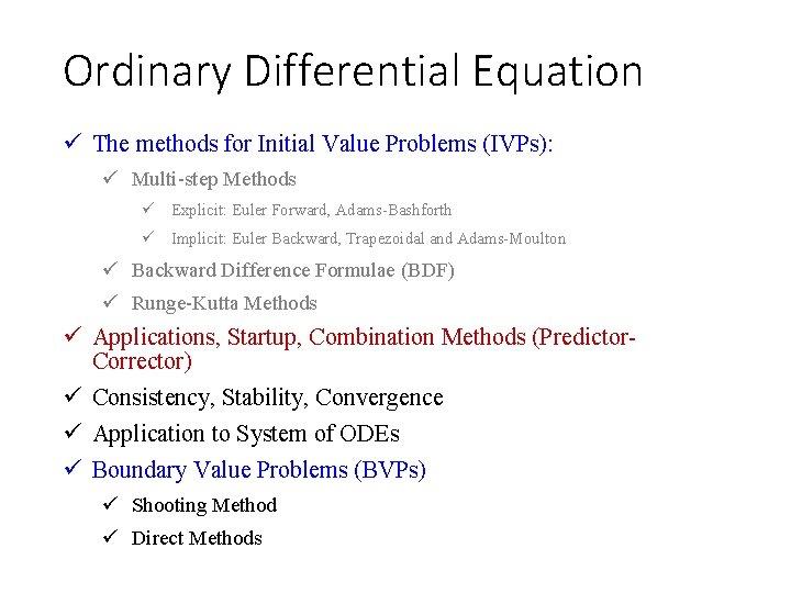
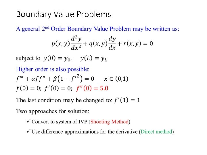
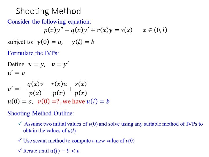
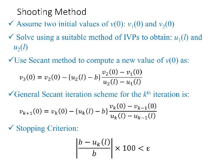
Ordinary Differential Equation ü The methods for Initial Value Problems (IVPs): ü Multi-step Methods ü Explicit: Euler Forward, Adams-Bashforth ü Implicit: Euler Backward, Trapezoidal and Adams-Moulton ü Backward Difference Formulae (BDF) ü Runge-Kutta Methods ü Applications, Startup, Combination Methods (Predictor. Corrector) ü Consistency, Stability, Convergence ü Application to System of ODEs ü Boundary Value Problems (BVPs) ü Shooting Method ü Direct Methods

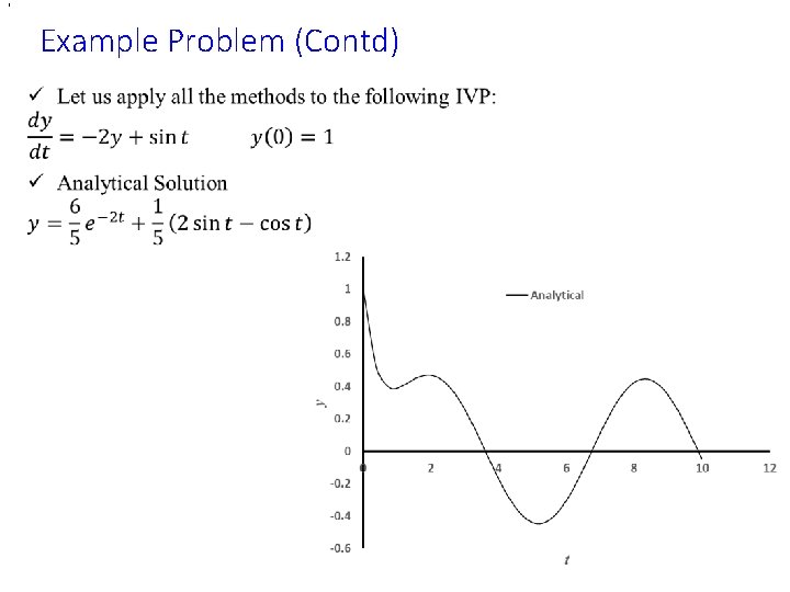
, Example Problem (Contd) •

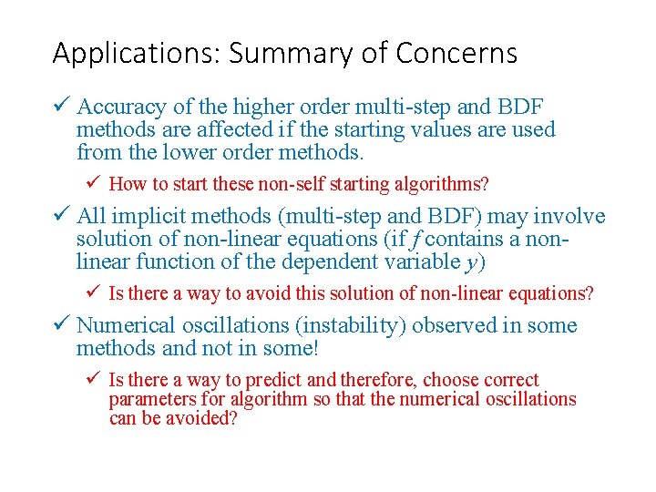
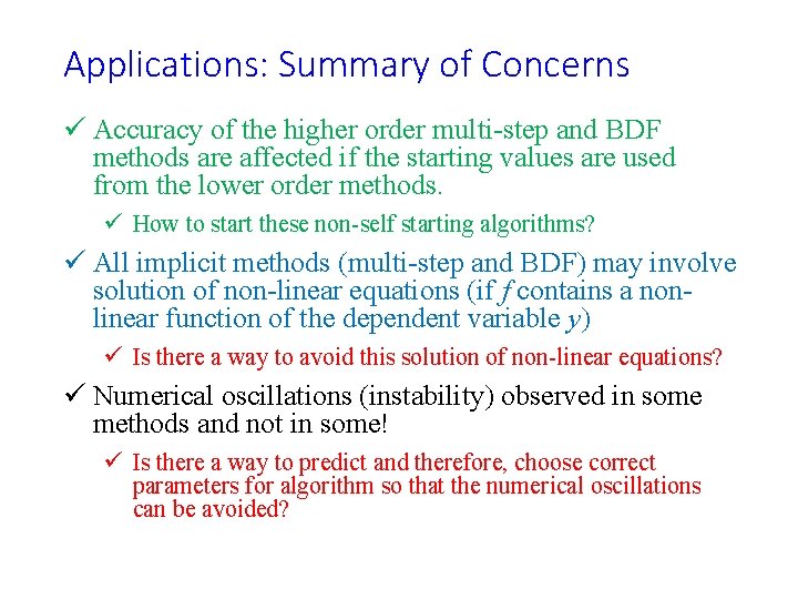
Applications: Summary of Concerns ü Accuracy of the higher order multi-step and BDF methods are affected if the starting values are used from the lower order methods. ü How to start these non-self starting algorithms? ü All implicit methods (multi-step and BDF) may involve solution of non-linear equations (if f contains a nonlinear function of the dependent variable y) ü Is there a way to avoid this solution of non-linear equations? ü Numerical oscillations (instability) observed in some methods and not in some! ü Is there a way to predict and therefore, choose correct parameters for algorithm so that the numerical oscillations can be avoided?

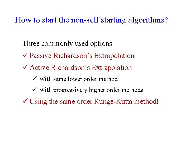
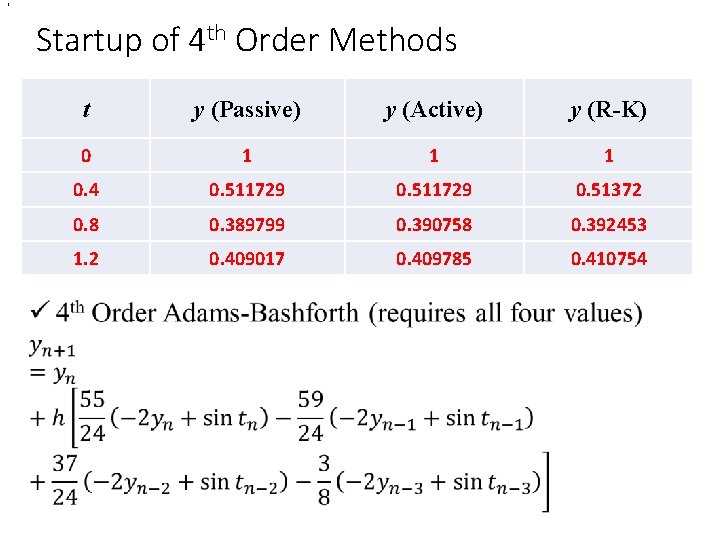
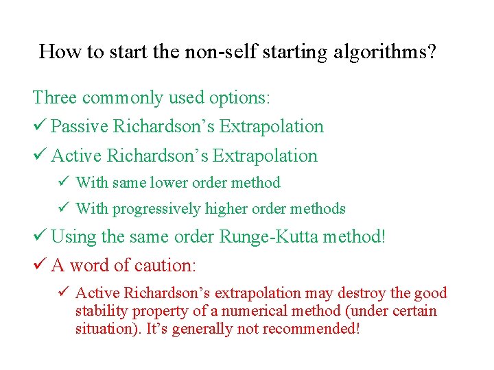
How to start the non-self starting algorithms? Three commonly used options: ü Passive Richardson’s Extrapolation ü Active Richardson’s Extrapolation ü With same lower order method ü With progressively higher order methods ü Using the same order Runge-Kutta method!

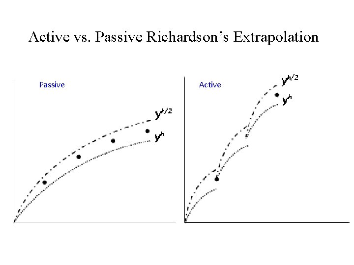
Active vs. Passive Richardson’s Extrapolation Passive Active

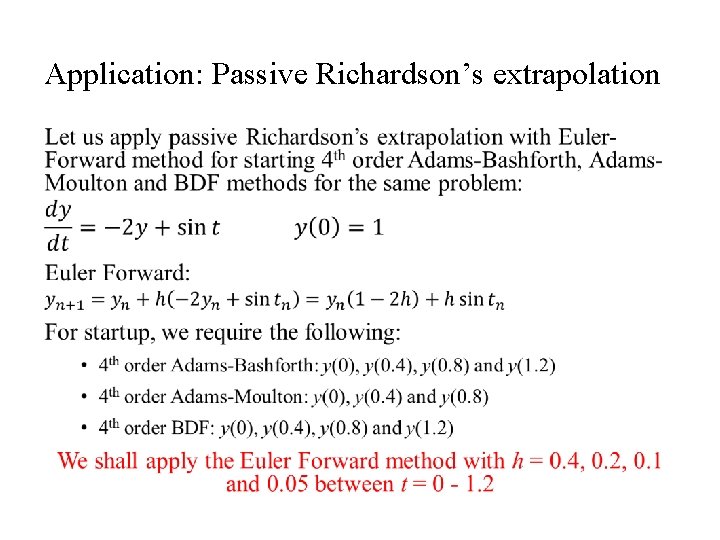
Application: Passive Richardson’s extrapolation •

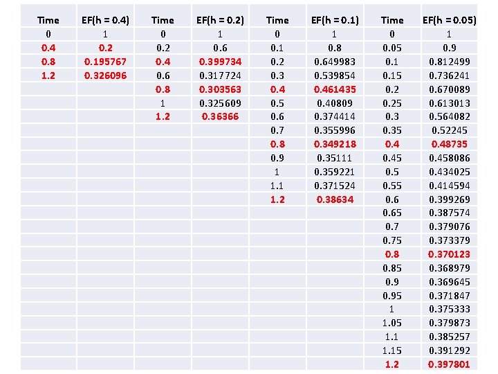
Time 0 0. 4 0. 8 1. 2 EF(h = 0. 4) 1 0. 2 0. 195767 0. 326096 Time 0 0. 2 0. 4 0. 6 0. 8 1 1. 2 EF(h = 0. 2) 1 0. 6 0. 399734 0. 317724 0. 303563 0. 325609 0. 36366 Time 0 0. 1 0. 2 0. 3 0. 4 0. 5 0. 6 0. 7 0. 8 0. 9 1 1. 2 EF(h = 0. 1) 1 0. 8 0. 649983 0. 539854 0. 461435 0. 40809 0. 374414 0. 355996 0. 349218 0. 35111 0. 359221 0. 371524 0. 38634 Time 0 0. 05 0. 15 0. 25 0. 35 0. 45 0. 55 0. 65 0. 75 0. 85 0. 95 1 1. 05 1. 15 1. 2 EF(h = 0. 05) 1 0. 9 0. 812499 0. 736241 0. 670089 0. 613013 0. 564082 0. 52245 0. 48735 0. 458086 0. 434025 0. 414594 0. 399269 0. 387574 0. 379076 0. 373379 0. 370123 0. 368979 0. 369645 0. 371847 0. 375333 0. 379873 0. 385257 0. 391292 0. 397801

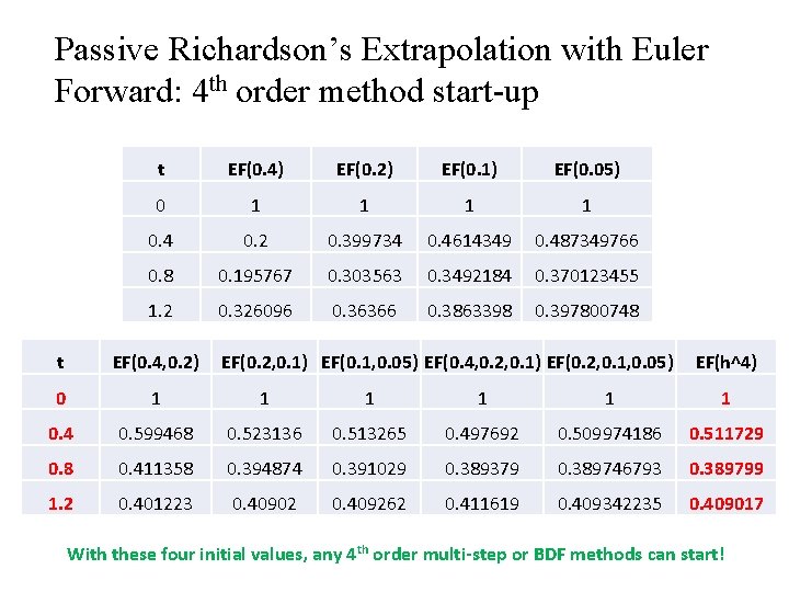
Passive Richardson’s Extrapolation with Euler Forward: 4 th order method start-up t EF(0. 4) EF(0. 2) EF(0. 1) EF(0. 05) 0 1 1 0. 4 0. 2 0. 399734 0. 4614349 0. 487349766 0. 8 0. 195767 0. 303563 0. 3492184 0. 370123455 1. 2 0. 326096 0. 36366 0. 3863398 0. 397800748 t EF(0. 4, 0. 2) EF(0. 2, 0. 1) EF(0. 1, 0. 05) EF(0. 4, 0. 2, 0. 1) EF(0. 2, 0. 1, 0. 05) EF(h^4) 0 1 1 1 0. 4 0. 599468 0. 523136 0. 513265 0. 497692 0. 509974186 0. 511729 0. 8 0. 411358 0. 394874 0. 391029 0. 389379 0. 389746793 0. 389799 1. 2 0. 401223 0. 40902 0. 409262 0. 411619 0. 409342235 0. 409017 With these four initial values, any 4 th order multi-step or BDF methods can start!

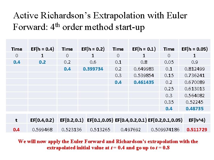
Active Richardson’s Extrapolation with Euler Forward: 4 th order method start-up Time 0 0. 4 EF(h = 0. 4) 1 0. 2 Time 0 0. 2 0. 4 EF(h = 0. 2) 1 0. 6 0. 399734 t EF(0. 4, 0. 2) EF(0. 2, 0. 1) EF(0. 1, 0. 05) EF(0. 4, 0. 2, 0. 1) EF(0. 2, 0. 1, 0. 05) 0. 4 0. 599468 0. 523136 0. 513265 Time 0 0. 1 0. 2 0. 3 0. 4 EF(h = 0. 1) 1 0. 8 0. 649983 0. 539854 0. 461435 0. 497692 Time 0 0. 05 0. 15 0. 25 0. 35 0. 4 0. 509974186 EF(h = 0. 05) 1 0. 9 0. 812499 0. 736241 0. 670089 0. 613013 0. 564082 0. 52245 0. 48735 EF(h^4) 0. 511729 We will now apply the Euler Forward and Richardson’s extrapolation with the extrapolated initial value at t = 0. 4 and go up to t = 0. 8

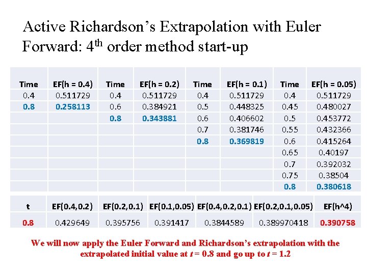
Active Richardson’s Extrapolation with Euler Forward: 4 th order method start-up Time 0. 4 0. 8 EF(h = 0. 4) 0. 511729 0. 258113 Time 0. 4 0. 6 0. 8 EF(h = 0. 2) 0. 511729 0. 384921 0. 343881 t EF(0. 4, 0. 2) EF(0. 2, 0. 1) EF(0. 1, 0. 05) EF(0. 4, 0. 2, 0. 1) EF(0. 2, 0. 1, 0. 05) 0. 8 0. 429649 0. 395756 0. 391417 Time 0. 4 0. 5 0. 6 0. 7 0. 8 EF(h = 0. 1) 0. 511729 0. 448325 0. 406602 0. 381746 0. 369819 0. 3844589 Time 0. 45 0. 55 0. 65 0. 75 0. 8 0. 389970418 EF(h = 0. 05) 0. 511729 0. 480027 0. 453772 0. 432366 0. 415264 0. 40197 0. 392032 0. 38504 0. 380618 EF(h^4) 0. 390758 We will now apply the Euler Forward and Richardson’s extrapolation with the extrapolated initial value at t = 0. 8 and go up to t = 1. 2

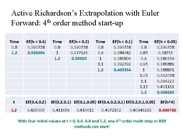
Active Richardson’s Extrapolation with Euler Forward: 4 th order method start-up Time 0. 8 1. 2 EF(h = 0. 4) 0. 390758 0. 365094 Time 0. 8 1 1. 2 EF(h = 0. 2) 0. 390758 0. 377926 0. 39505 t EF(0. 4, 0. 2) EF(0. 2, 0. 1) EF(0. 1, 0. 05) EF(0. 4, 0. 2, 0. 1) EF(0. 2, 0. 1, 0. 05) 1. 2 0. 425005 0. 411659 0. 410012 Time 0. 8 0. 9 1 1. 2 EF(h = 0. 1) 0. 390758 0. 384342 0. 385806 0. 392792 0. 403354 0. 4072102 Time 0. 85 0. 95 1 1. 05 1. 15 1. 2 0. 40946293 EF(h = 0. 05) 0. 390758 0. 38755 0. 386359 0. 386889 0. 388871 0. 392058 0. 396223 0. 401161 0. 406683 EF(h^4) 0. 409785 With four initial values at t = 0, 0. 4, 0. 8 and 1. 2, any 4 th order multi-step or BDF methods can start!

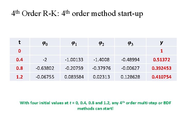
4 th Order R-K: 4 th order method start-up t φ0 φ1 φ2 φ3 0 y 1 0. 4 -2 -1. 00133 -1. 4008 -0. 48994 0. 51372 0. 8 -0. 63802 -0. 20759 -0. 37976 -0. 00627 0. 392453 1. 2 -0. 06755 0. 083584 0. 02313 0. 128628 0. 410754 With four initial values at t = 0, 0. 4, 0. 8 and 1. 2, any 4 th order multi-step or BDF methods can start!

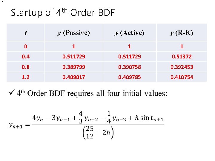
, Startup of 4 th Order Methods • t y (Passive) y (Active) y (R-K) 0 1 1 1 0. 4 0. 511729 0. 51372 0. 8 0. 389799 0. 390758 0. 392453 1. 2 0. 409017 0. 409785 0. 410754

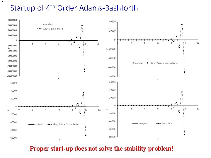
, Startup of 4 th Order Adams-Bashforth Proper start-up does not solve the stability problem!

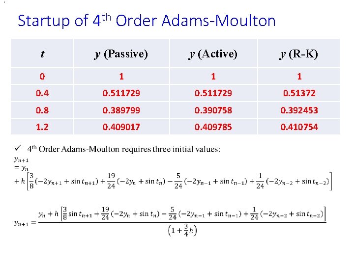
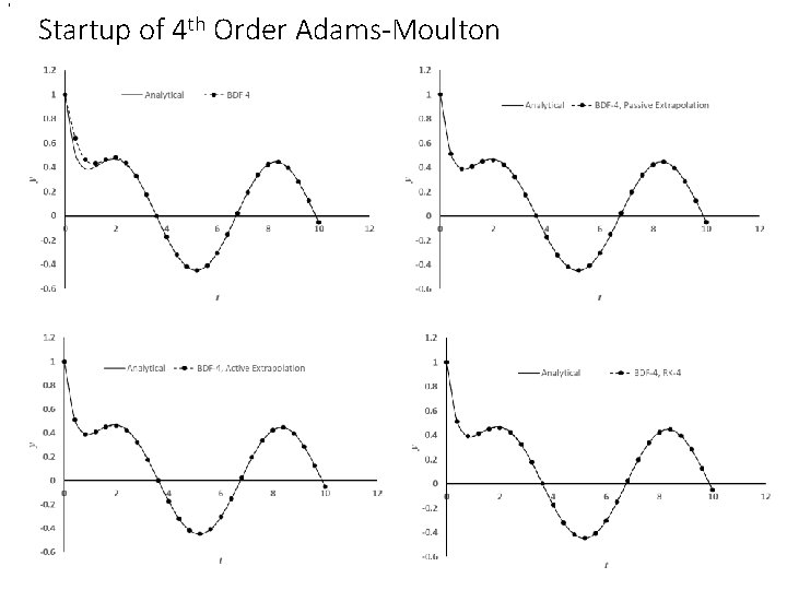
, Startup of 4 th Order Adams-Moulton • t y (Passive) y (Active) y (R-K) 0 1 1 1 0. 4 0. 511729 0. 51372 0. 8 0. 389799 0. 390758 0. 392453 1. 2 0. 409017 0. 409785 0. 410754

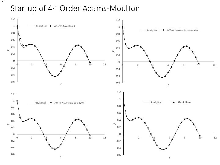
, Startup of 4 th Order Adams-Moulton

, Startup of 4 th Order BDF • t y (Passive) y (Active) y (R-K) 0 1 1 1 0. 4 0. 511729 0. 51372 0. 8 0. 389799 0. 390758 0. 392453 1. 2 0. 409017 0. 409785 0. 410754

, Startup of 4 th Order Adams-Moulton

How to start the non-self starting algorithms? Three commonly used options: ü Passive Richardson’s Extrapolation ü Active Richardson’s Extrapolation ü With same lower order method ü With progressively higher order methods ü Using the same order Runge-Kutta method! ü A word of caution: ü Active Richardson’s extrapolation may destroy the good stability property of a numerical method (under certain situation). It’s generally not recommended!

Applications: Summary of Concerns ü Accuracy of the higher order multi-step and BDF methods are affected if the starting values are used from the lower order methods. ü How to start these non-self starting algorithms? ü All implicit methods (multi-step and BDF) may involve solution of non-linear equations (if f contains a nonlinear function of the dependent variable y) ü Is there a way to avoid this solution of non-linear equations? ü Numerical oscillations (instability) observed in some methods and not in some! ü Is there a way to predict and therefore, choose correct parameters for algorithm so that the numerical oscillations can be avoided?

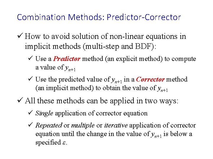
Combination Methods: Predictor-Corrector ü How to avoid solution of non-linear equations in implicit methods (multi-step and BDF): ü Use a Predictor method (an explicit method) to compute a value of yn+1 ü Use the predicted value of yn+1 in a Corrector method (an implicit method) to obtain the value of yn+1 ü All these methods can be applied in two ways: ü Single application of corrector equation ü Repeated or multiple or iterative application of corrector equation until the change in the value of yn+1 is below a specified ε.

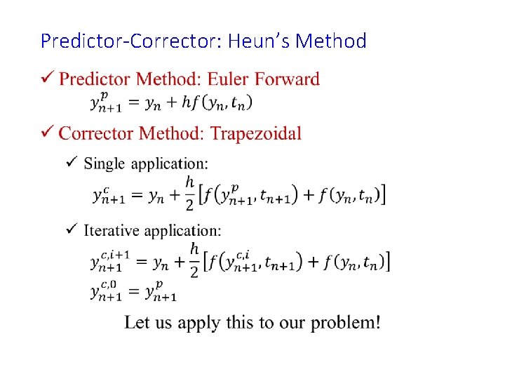
Predictor-Corrector: Heun’s Method •

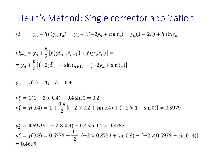
Heun’s Method: Single corrector application •

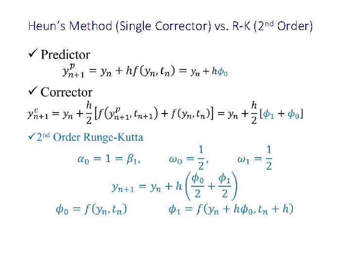
Heun’s Method (Single Corrector) vs. R-K (2 nd Order) •

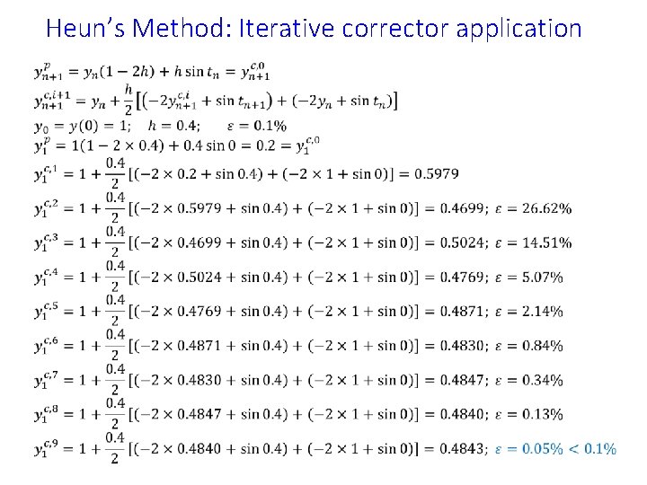
Heun’s Method: Iterative corrector application •

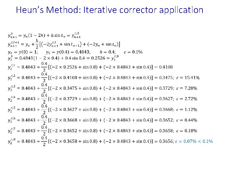
Heun’s Method: Iterative corrector application •

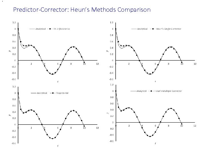
, Predictor-Corrector: Heun’s Methods Comparison

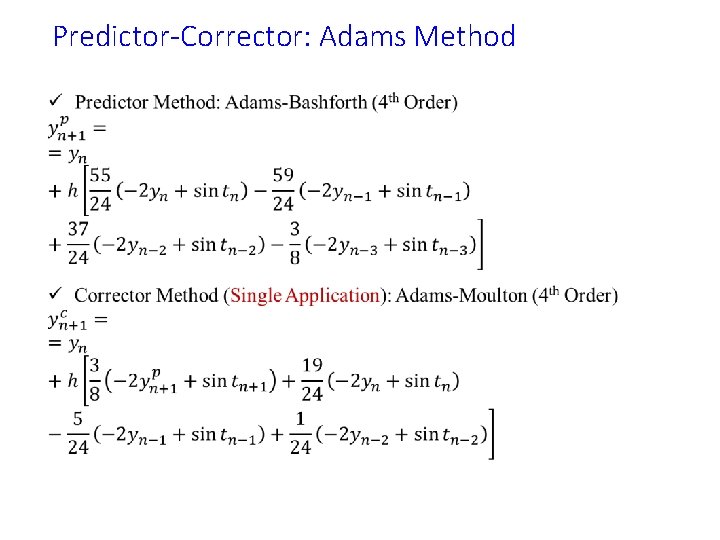
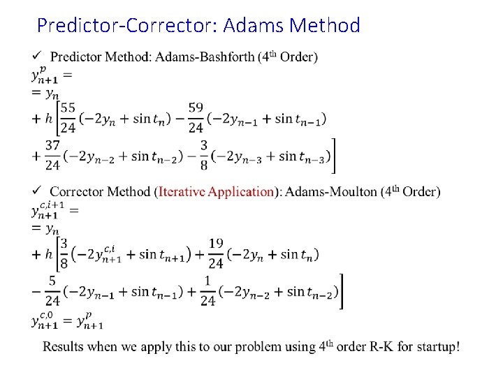
Predictor-Corrector: Adams Method •

Predictor-Corrector: Adams Method •

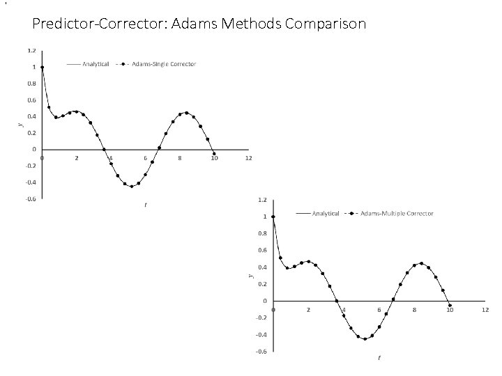
, Predictor-Corrector: Adams Methods Comparison

Combination Methods: Predictor-Corrector ü Predictor-Corrector methods only avoid the solution of non-linear equation. They still require appropriate startup to produce proper results! ü Predictor-Corrector method have the same stability properties as the corrector method ü Adams-Bashforth (4 th order) was unstable for this problem with h = 0. 4 but the predictor-corrector method produced correct results because of the influence of the corrector method Adams-Moulton (4 th order), which was stable! ü Iterative application of corrector produces more accurate results but at the expense of higher FLOPs.

Applications: Summary of Concerns ü Accuracy of the higher order multi-step and BDF methods are affected if the starting values are used from the lower order methods. ü How to start these non-self starting algorithms? ü All implicit methods (multi-step and BDF) may involve solution of non-linear equations (if f contains a nonlinear function of the dependent variable y) ü Is there a way to avoid this solution of non-linear equations? ü Numerical oscillations (instability) observed in some methods and not in some! ü Is there a way to predict and therefore, choose correct parameters for algorithm so that the numerical oscillations can be avoided? We will do Convergence Analysis!

ESO 208 A: Computational Methods in Engineering Ordinary Differential Equation: Boundary Value Problems Abhas Singh Department of Civil Engineering IIT Kanpur Acknowledgements: Profs. Saumyen Guha and Shivam Tripathi (CE)

Boundary Value Problems •

Shooting Method •

Shooting Method •

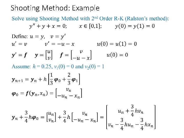
Shooting Method: Example •

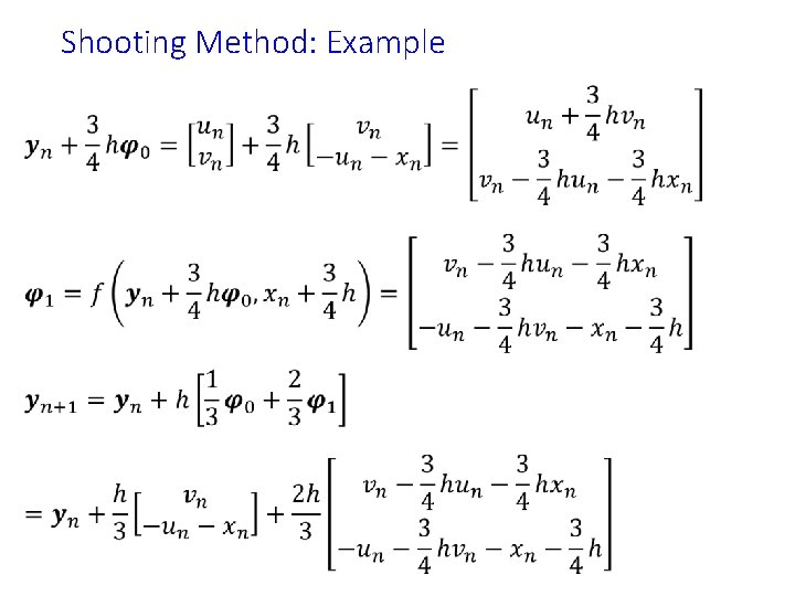
• Shooting Method: Example

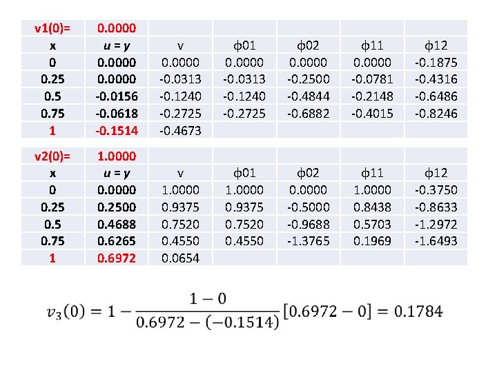
v 1(0)= x 0 0. 25 0. 75 1 0. 0000 u=y 0. 0000 -0. 0156 -0. 0618 -0. 1514 v 0. 0000 -0. 0313 -0. 1240 -0. 2725 -0. 4673 φ01 0. 0000 -0. 0313 -0. 1240 -0. 2725 φ02 0. 0000 -0. 2500 -0. 4844 -0. 6882 φ11 0. 0000 -0. 0781 -0. 2148 -0. 4015 φ12 -0. 1875 -0. 4316 -0. 6486 -0. 8246 v 2(0)= x 0 0. 25 0. 75 1 1. 0000 u=y 0. 0000 0. 2500 0. 4688 0. 6265 0. 6972 v 1. 0000 0. 9375 0. 7520 0. 4550 0. 0654 φ01 1. 0000 0. 9375 0. 7520 0. 4550 φ02 0. 0000 -0. 5000 -0. 9688 -1. 3765 φ11 1. 0000 0. 8438 0. 5703 0. 1969 φ12 -0. 3750 -0. 8633 -1. 2972 -1. 6493

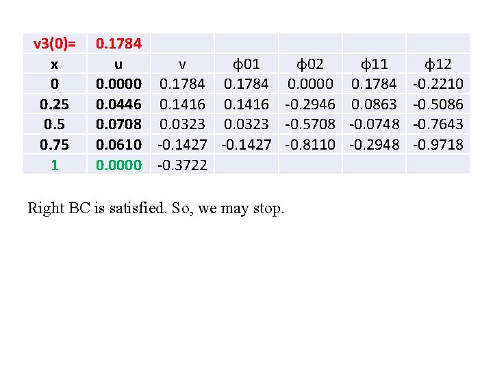
v 3(0)= x 0 0. 25 0. 75 1 0. 1784 u v 0. 0000 0. 1784 0. 0446 0. 1416 0. 0708 0. 0323 0. 0610 -0. 1427 0. 0000 -0. 3722 φ01 0. 1784 0. 1416 0. 0323 -0. 1427 Right BC is satisfied. So, we may stop. φ02 0. 0000 -0. 2946 -0. 5708 -0. 8110 φ11 0. 1784 0. 0863 -0. 0748 -0. 2948 φ12 -0. 2210 -0. 5086 -0. 7643 -0. 9718

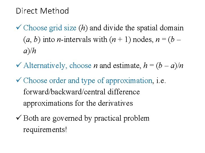
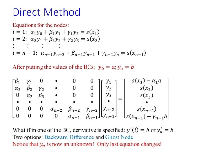
Direct Method ü Choose grid size (h) and divide the spatial domain (a, b) into n-intervals with (n + 1) nodes, n = (b – a)/h ü Alternatively, choose n and estimate, h = (b – a)/n ü Choose order and type of approximation, i. e. forward/backward/central difference approximations for the derivatives ü Both are governed by practical problem requirements!

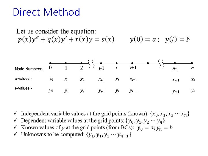
Direct Method

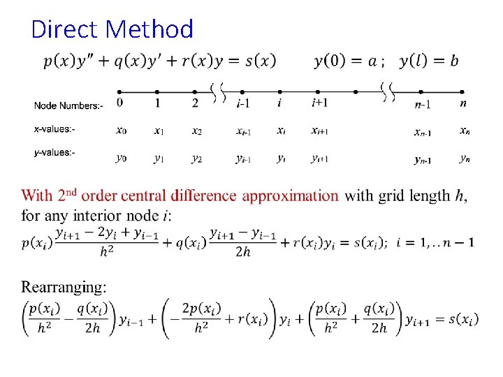
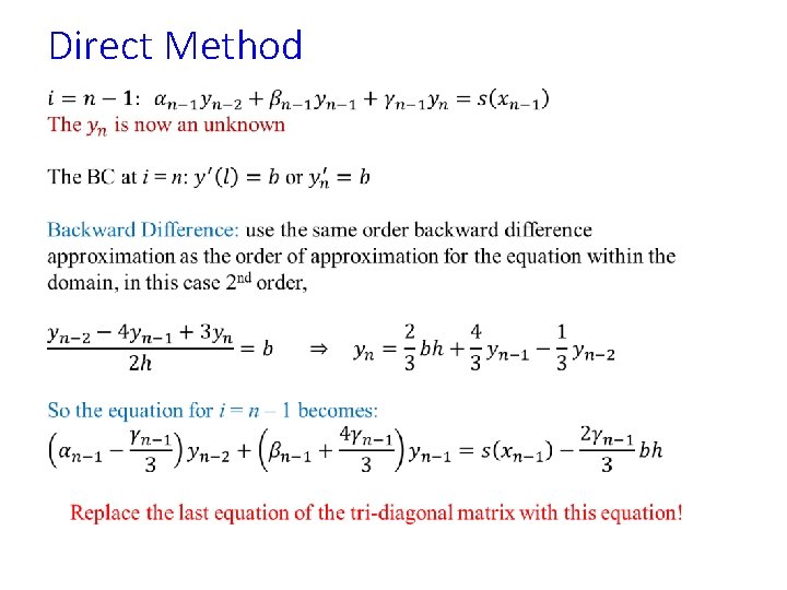
Direct Method

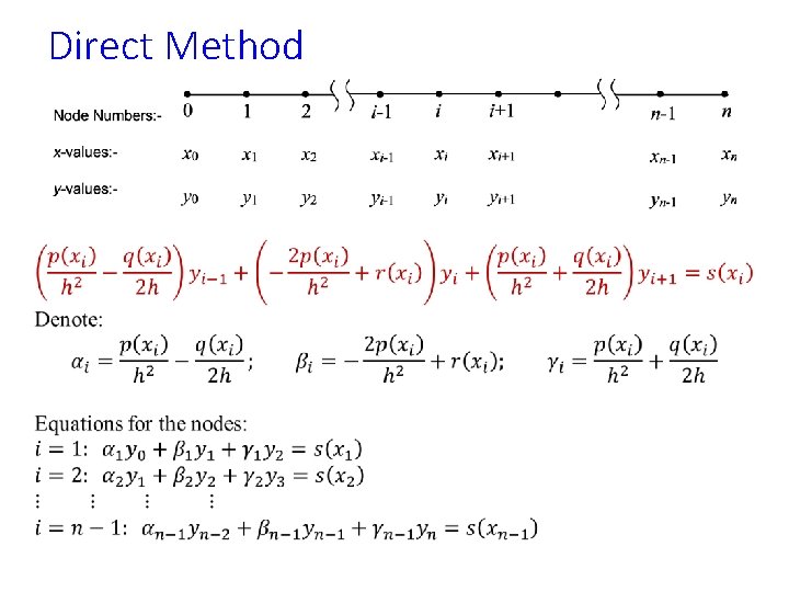
Direct Method

Direct Method

Direct Method

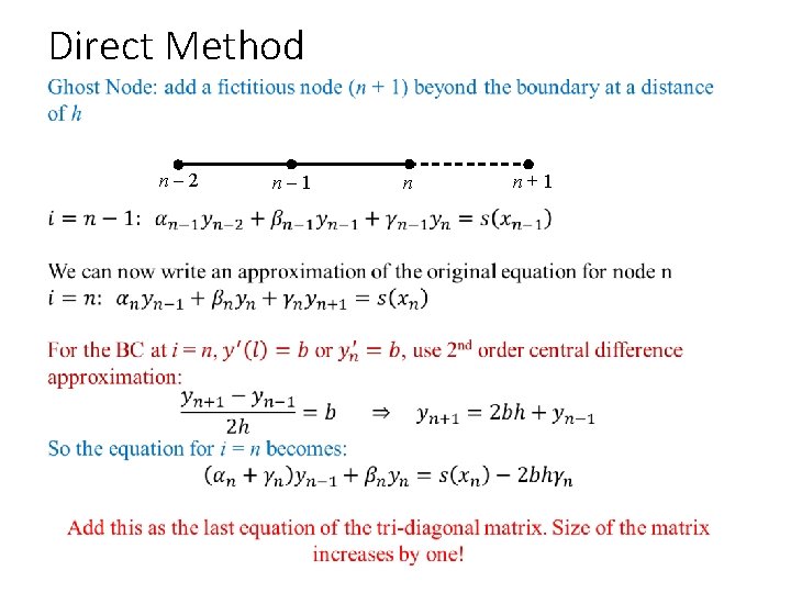
Direct Method n– 2 n– 1 n n+1

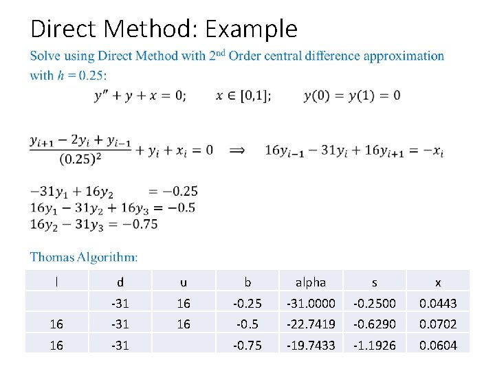
Direct Method: Example l d u b alpha s x -31 16 -0. 25 -31. 0000 -0. 2500 0. 0443 16 -31 16 -0. 5 -22. 7419 -0. 6290 0. 0702 16 -31 -0. 75 -19. 7433 -1. 1926 0. 0604

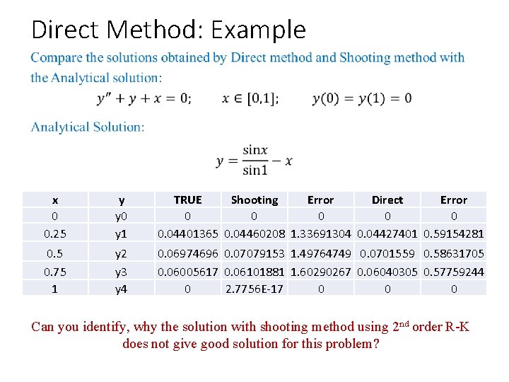
Direct Method: Example x 0 0. 25 y y 0 y 1 TRUE Shooting Error Direct Error 0 0 0. 04401365 0. 04460208 1. 33691304 0. 04427401 0. 59154281 0. 5 0. 75 1 y 2 y 3 y 4 0. 06974696 0. 07079153 1. 49764749 0. 0701559 0. 58631705 0. 06005617 0. 06101881 1. 60290267 0. 06040305 0. 57759244 0 2. 7756 E-17 0 0 0 Can you identify, why the solution with shooting method using 2 nd order R-K does not give good solution for this problem?