Ordinal Logistic Regression By Ahlam Lee Contents Concepts

Ordinal Logistic Regression By Ahlam Lee

Contents • • • Concepts of Ordinal Logistic Regression Assumptions of Ordinal Logistic Regression Our research Question SPSS demonstration SPSS outputs and interpretation

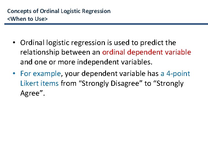
Concepts of Ordinal Logistic Regression <When to Use> • Ordinal logistic regression is used to predict the relationship between an ordinal dependent variable and one or more independent variables. • For example, your dependent variable has a 4 -point Likert items from “Strongly Disagree” to “Strongly Agree”.

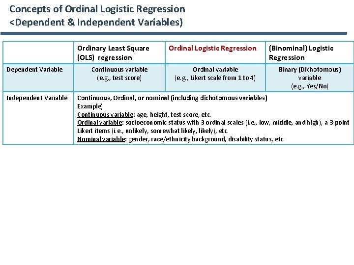
Concepts of Ordinal Logistic Regression <Dependent & Independent Variables) Dependent Variable Independent Variable Ordinary Least Square (OLS) regression Ordinal Logistic Regression Continuous variable (e. g. , test score) Ordinal variable (e. g. , Likert scale from 1 to 4) (Binominal) Logistic Regression Binary (Dichotomous) variable (e. g. , Yes/No) Continuous, Ordinal, or nominal (including dichotomous variables) Example) Continuous variable: age, height, test score, etc. Ordinal variable: socioeconomic status with 3 ordinal scales (i. e. , low, middle, and high), a 3 -point Likert items (i. e. , unlikely, somewhat likely, likely), etc. Nominal variable: gender, race/ethnicity background, disability status, etc.

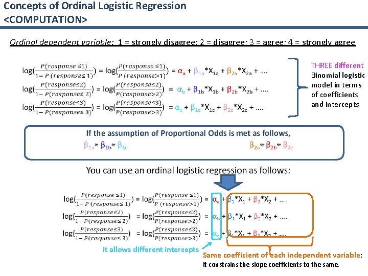
Concepts of Ordinal Logistic Regression <COMPUTATION> Ordinal dependent variable: 1 = strongly disagree; 2 = disagree; 3 = agree; 4 = strongly agree THREE different Binomial logistic model in terms of coefficients and intercepts • It allows different intercepts Same coefficient of each independent variable: It constrains the slope coefficients to the same.

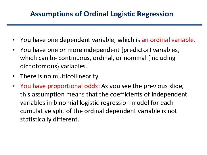
Assumptions of Ordinal Logistic Regression • You have one dependent variable, which is an ordinal variable. • You have one or more independent (predictor) variables, which can be continuous, ordinal, or nominal (including dichotomous) variables. • There is no multicollinearity • You have proportional odds: As you see the previous slide, this assumption means that the coefficients of independent variables in binomial logistic regression model for each cumulative split of the ordinal dependent variable is not statistically different.

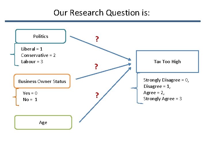
Our Research Question is: Politics Liberal = 1 Conservative = 2 Labour = 3 ? ? Business Owner Status Yes = 0 No = 1 ? Age Tax Too High Strongly Disagree = 0, Disagree = 1, Agree = 2, Strongly Agree = 3

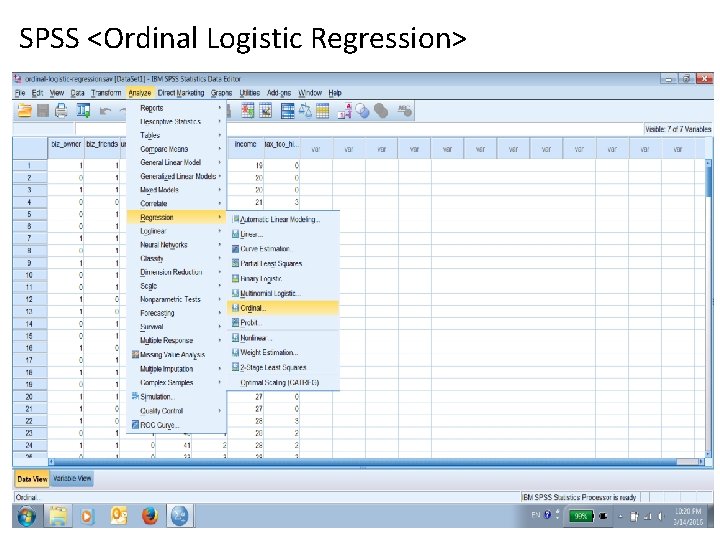
SPSS <Ordinal Logistic Regression>

SPSS <Ordinal Logistic Regression>

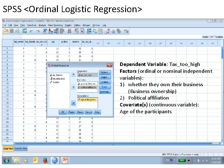
SPSS <Ordinal Logistic Regression> Dependent Variable: Tax_too_high Factors (ordinal or nominal independent variables): 1) whether they own their business (Business ownership) 2) Political affiliation Covariate(s) (continuous variable): Age of the participants

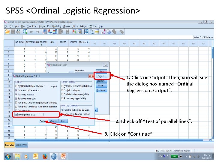
SPSS <Ordinal Logistic Regression> 1. Click on Output. Then, you will see the dialog box named “Ordinal Regression: Output”. 2. Check off “Test of parallel lines”. 3. Click on “Continue”.

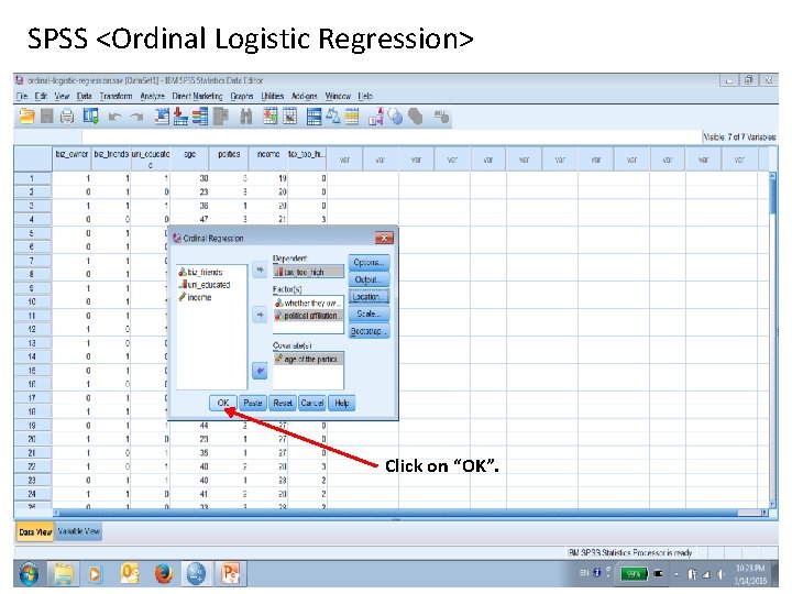
SPSS <Ordinal Logistic Regression> Click on “OK”.

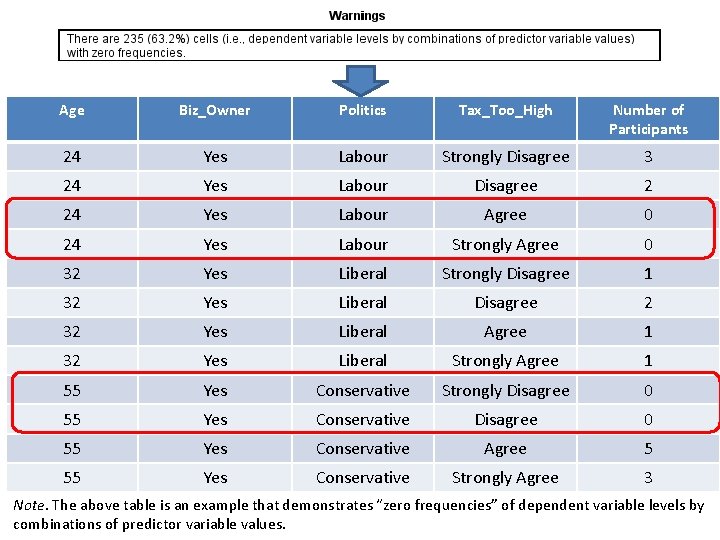
Age Biz_Owner Politics Tax_Too_High Number of Participants 24 Yes Labour Strongly Disagree 3 24 Yes Labour Disagree 2 24 Yes Labour Agree 0 24 Yes Labour Strongly Agree 0 32 Yes Liberal Strongly Disagree 1 32 Yes Liberal Disagree 2 32 Yes Liberal Agree 1 32 Yes Liberal Strongly Agree 1 55 Yes Conservative Strongly Disagree 0 55 Yes Conservative Agree 5 55 Yes Conservative Strongly Agree 3 Note. The above table is an example that demonstrates “zero frequencies” of dependent variable levels by combinations of predictor variable values.

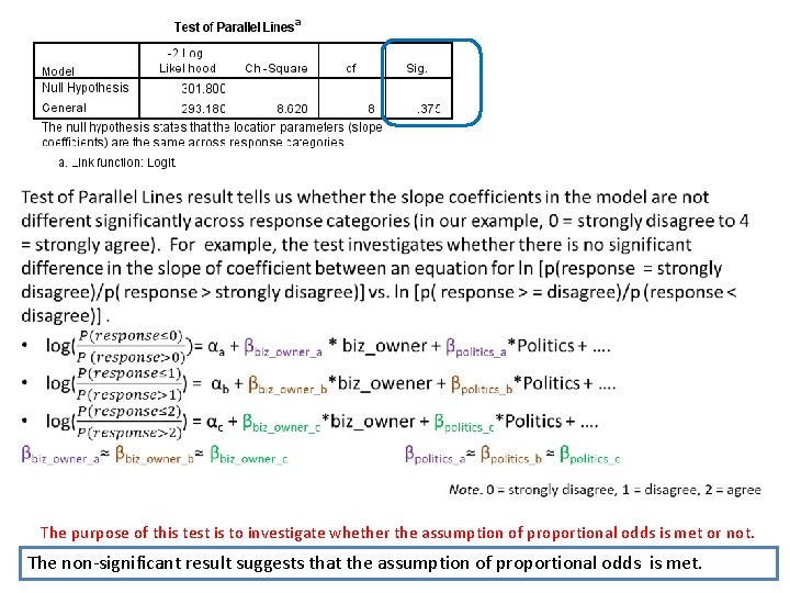
The purpose of this test is to investigate whether the assumption of proportional odds is met or not. The non-significant result suggests that the assumption of proportional odds is met.

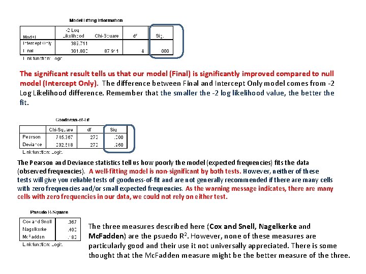
The significant result tells us that our model (Final) is significantly improved compared to null model (Intercept Only). The difference between Final and Intercept Only model comes from -2 Log Likelihood difference. Remember that the smaller the -2 log likelihood value, the better the fit. The Pearson and Deviance statistics tell us how poorly the model (expected frequencies) fits the data (observed frequencies). A well-fitting model is non-significant by both tests. However, neither of these tests will give you reliable tests of goodness-of-fit and are not generally recommended if there are many cells with zero frequencies and/or small expected frequencies. As the warning message indicates, there are many cells with zero frequencies in our data, we could not rely on either test. The three measures described here (Cox and Snell, Nagelkerke and Mc. Fadden) are the psuedo R 2. However, none of these measures are particularly good and their use it not universally appreciated. There is some thought that the Mc. Fadden measure might be the better measure of the three.

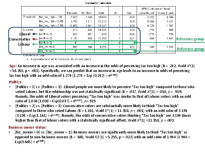
Liberal Conservative Labour Reference group Age: An increase in age was associated with an increase in the odds of perceiving tax too high (B =. 242, Wald X 2(1) = 56. 355, p <. 001). Specifically, we can predict that an increase in age leads to an increase in odds of perceiving tax too high with an odd ratio of 1. 274 (1. 274 = Exp (0. 242) = e 0. 242) Politics: • [Politics = 1] vs. [Politics = 3]: Liberal people are more likely to perceive “Tax too high” compared to those who voted Labour, but the relationship was not statistically significant (B =. 037, Wald X 2(1) =. 010, p =. 919). Namely, the odds of Liberal voters perceiving “Tax too high” was similar to that of Labour voters with an odd ratio of 1. 038 (1. 038 = Exp(0. 037) = e 0. 037), p=. 919. • [Politics = 2] vs. [Politics = 3]: Conservative voters are substantially more likely to think “Tax too high” compared to those who voted Labour (B = 1. 161, Wald X 2 (1) = 11. 358, p =. 001) with an odd ratio of 3. 194 (3. 194 = Exp(1. 161) = e 1. 161). Namely, the odds of conservative voters thinking “Tax too high” are 3. 194 times higher than that of labour voters with a statistically significant effect, Wald X 2(1) =11. 358, p =. 001. Business owner status: • [biz_owner = 0] vs. [biz_owner = 1]: Business owners are significantly more likely to think “Tax too high” as opposed to non-business owners (B =. 665, Wald X 2 (1) = 5. 255, p =. 022) with an odd ratio of 1. 944 (1. 944 = Exp(0. 665) = e 0. 665).

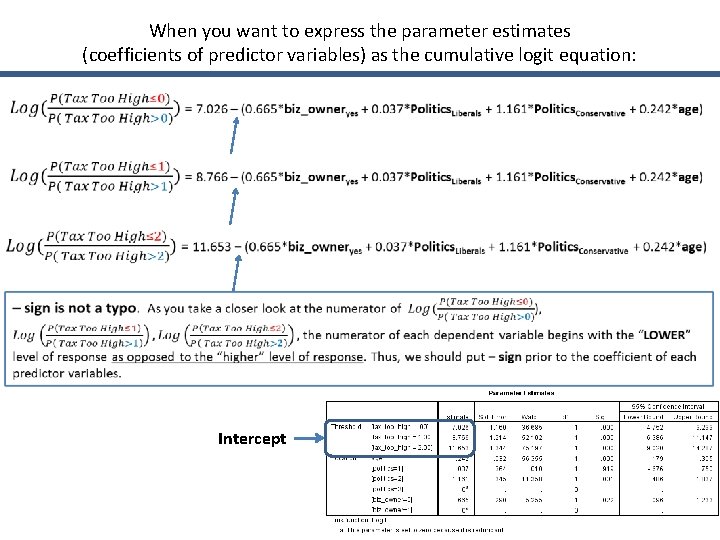
When you want to express the parameter estimates (coefficients of predictor variables) as the cumulative logit equation: Intercept

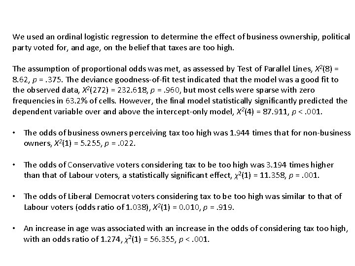
We used an ordinal logistic regression to determine the effect of business ownership, political party voted for, and age, on the belief that taxes are too high. The assumption of proportional odds was met, as assessed by Test of Parallel Lines, X 2(8) = 8. 62, p =. 375. The deviance goodness-of-fit test indicated that the model was a good fit to the observed data, X 2(272) = 232. 618, p =. 960, but most cells were sparse with zero frequencies in 63. 2% of cells. However, the final model statistically significantly predicted the dependent variable over and above the intercept-only model, X 2(4) = 87. 911, p <. 001. • The odds of business owners perceiving tax too high was 1. 944 times that for non-business owners, X 2(1) = 5. 255, p =. 022. • The odds of Conservative voters considering tax to be too high was 3. 194 times higher than that of Labour voters, a statistically significant effect, χ2(1) = 11. 358, p =. 001. • The odds of Liberal Democrat voters considering tax to be too high was similar to that of Labour voters (odds ratio of 1. 038), X 2(1) = 0. 010, p =. 919. • An increase in age was associated with an increase in the odds of considering tax too high, with an odds ratio of 1. 274, χ2(1) = 56. 355, p <. 001.