ORDINAL AND SEQUENTIAL LOGIT MODELS DISCRETE CHOICE MODELING

ORDINAL AND SEQUENTIAL LOGIT MODELS DISCRETE CHOICE MODELING IN HEALTH ECONOMICS COPYRIGHT OF: ABHINAV ANAND JYOTI ARORA SHRADDHA RAMSWAMY

INTRODUCTION �Studies suggest that self rated health score is a reliable predictor of health status We investigate impact of a host of personal and status characteristics such as age, gender etc on the health perception of US Citizens

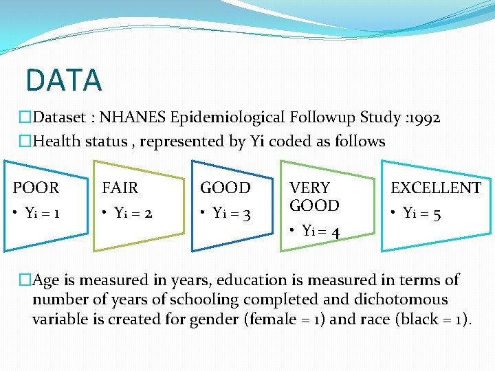
DATA �Dataset : NHANES Epidemiological Followup Study : 1992 �Health status , represented by Yi coded as follows POOR • Yi = 1 FAIR • Yi = 2 GOOD • Yi = 3 VERY GOOD • Yi = 4 EXCELLENT • Yi = 5 �Age is measured in years, education is measured in terms of number of years of schooling completed and dichotomous variable is created for gender (female = 1) and race (black = 1).

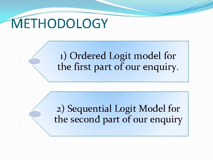
METHODOLOGY 1) Ordered Logit model for the first part of our enquiry. 2) Sequential Logit Model for the second part of our enquiry

ORDERED LOGIT MODEL SPECIFICATION �A multinomial choice model where the values taken by the dependent variable takes a natural order. 5 �Yi* is latent variable such that �Yi = j when αj-1 < Yi*< αj where j= 1, 2, 3, 4, 5 and �Yi* = β’Xi + ui where u follows logistic distribution. α 1 α 2 α 3 α 4

ORDERED LOGIT MODEL Where F( ) is a cdf and j = 1, 2, 3, 4, 5 and i is theith individual We assume that u follows logistic distribution

CONTD…. �P(Yi =1/Xi ) = F [ α 1 – β’X] �P(Yi = 2/Xi) = F [α 2 – β’X] – F[α 1 -β’X] �P(Yi = 3/Xi) = F [α 3 – β’X] – F [α 2 -β’X] �P(Yi = 4/Xi) = F [α 4– β’X] – F [α 3 – β’X] �P(Yi = 5/Xi) = 1– F [α 4 -β’X] Where F ( ) is defined as above. �For estimating the model we specify 5 dummy variables for the ith individual with the following rule �Zij = 1 if Yi = j where j = 1, 2, 3, 4, 5. = 0 otherwise

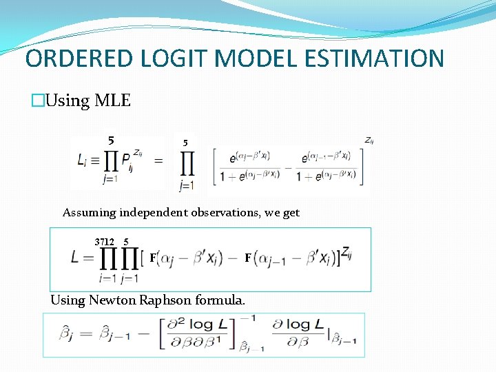
ORDERED LOGIT MODEL ESTIMATION �Using MLE 5 5 Assuming independent observations, we get 3712 5 F F Using Newton Raphson formula.

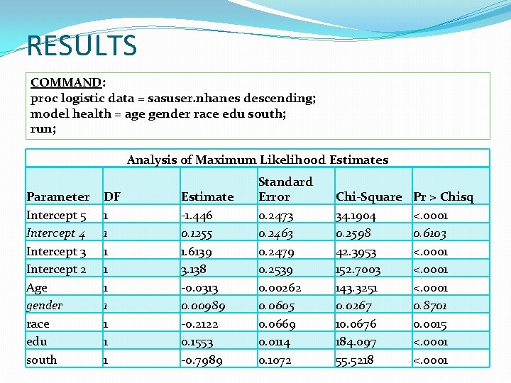
RESULTS COMMAND: proc logistic data = sasuser. nhanes descending; model health = age gender race edu south; run; Analysis of Maximum Likelihood Estimates Parameter Intercept 5 Intercept 4 Intercept 3 Intercept 2 Age gender race edu south DF 1 1 1 1 1 Estimate -1. 446 0. 1255 1. 6139 3. 138 -0. 0313 0. 00989 -0. 2122 0. 1553 -0. 7989 Standard Error 0. 2473 0. 2463 0. 2479 0. 2539 0. 00262 0. 0605 0. 0669 0. 0114 0. 1072 Chi-Square 34. 1904 0. 2598 42. 3953 152. 7003 143. 3251 0. 0267 10. 0676 184. 097 55. 5218 Pr > Chisq <. 0001 0. 6103 <. 0001 0. 8701 0. 0015 <. 0001

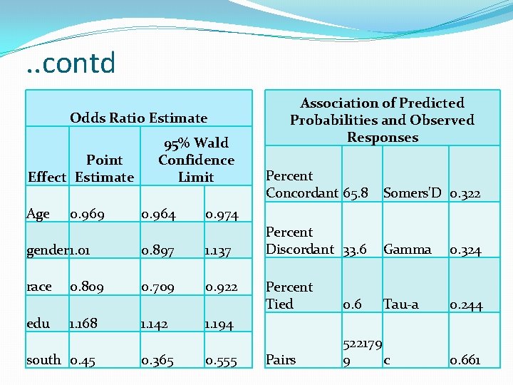
. . contd Odds Ratio Estimate Point Effect Estimate Age 0. 969 95% Wald Confidence Limit 0. 964 0. 897 1. 137 race 0. 709 0. 922 edu 1. 168 south 0. 45 1. 142 0. 365 Percent Concordant 65. 8 Somers'D 0. 322 Percent Discordant 33. 6 Gamma 0. 324 Percent Tied 0. 6 Tau-a 0. 244 Pairs 522179 9 c 0. 974 gender 1. 01 0. 809 Association of Predicted Probabilities and Observed Responses 1. 194 0. 555 0. 661

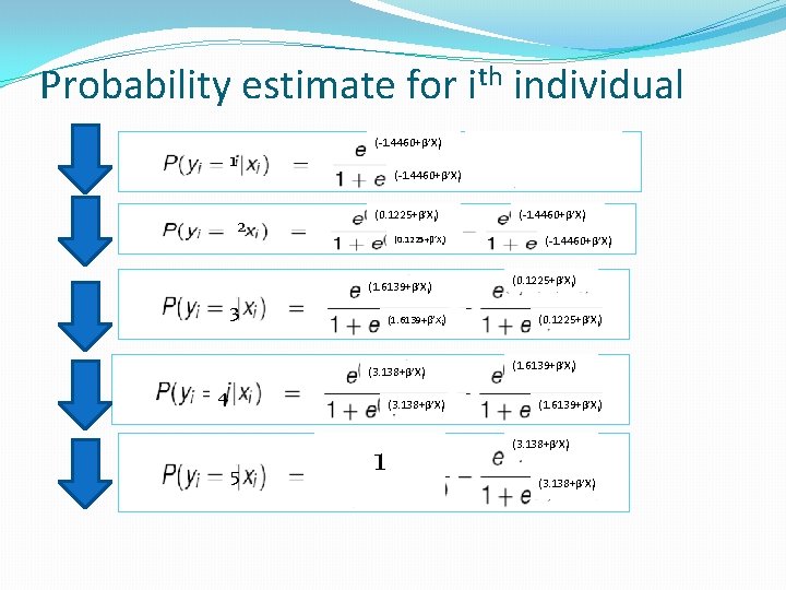
Probability estimate for ith individual (-1. 4460+β’X i) 1 (-1. 4460+β’X i) 2 (0. 1225+β’X i) (0. 1225+β’Xi) (1. 6139+β’X i) 3 (1. 6139+β’X i) (3. 138+β’X i) 4 (3. 138+β’X i) 5 1 (-1. 4460+β’X i) (0. 1225+β’X i) (1. 6139+β’X i) (3. 138+β’X i)

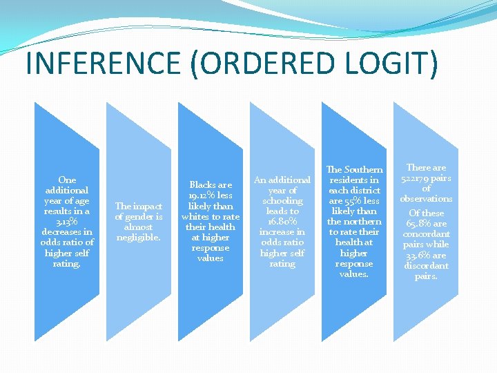
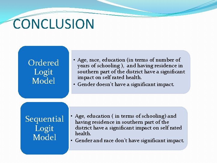
INFERENCE (ORDERED LOGIT) One additional year of age results in a 3. 13% decreases in odds ratio of higher self rating. The impact of gender is almost negligible. Blacks are 19. 12% less likely than whites to rate their health at higher response values An additional year of schooling leads to 16. 80% increase in odds ratio higher self rating The Southern residents in each district are 55% less likely than the northern to rate their health at higher response values. There are 522179 pairs of observations Of these 65. 8% are concordant pairs while 33. 6% are discordant pairs.

SEQUENTIAL LOGIT MODEL �Choices/Responses follow a sequence, so we need (m-1) latent variables to characterize (m) unordered choices. �Self-rated health measure can be considered as a purely cardinal variable following a sequence instead of some natural ordering. This allows us to perform discrete choice analysis using (non-ordered) sequential logit model.

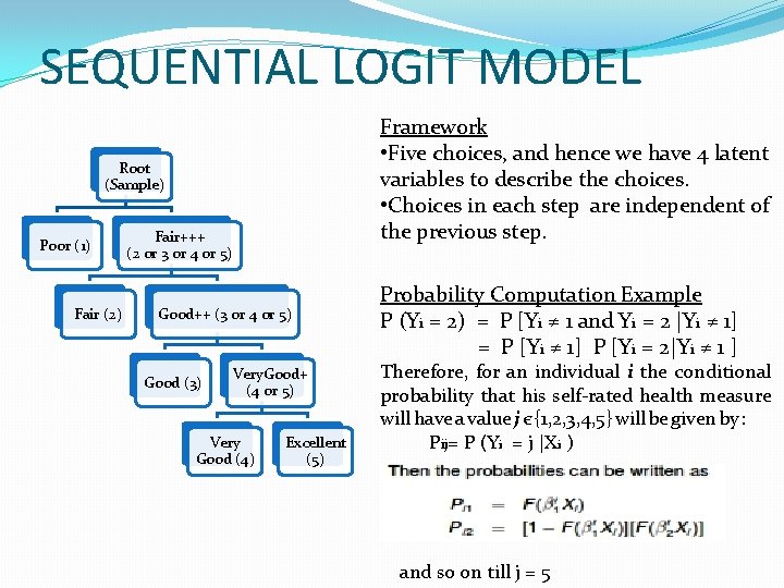
SEQUENTIAL LOGIT MODEL Framework • Five choices, and hence we have 4 latent variables to describe the choices. • Choices in each step are independent of the previous step. Root (Sample) Poor (1) Fair (2) Fair+++ (2 or 3 or 4 or 5) Good++ (3 or 4 or 5) Good (3) Very. Good+ (4 or 5) Very Good (4) Excellent (5) Probability Computation Example P (Yi = 2) = P [Yi ≠ 1 and Yi = 2 |Yi ≠ 1] = P [Yi ≠ 1] P [Yi = 2|Yi ≠ 1 ] Therefore, for an individual i the conditional probability that his self-rated health measure will have a value j є {1, 2, 3, 4, 5} will be given by : Pij= P (Yi = j |Xi ) and so on till j = 5

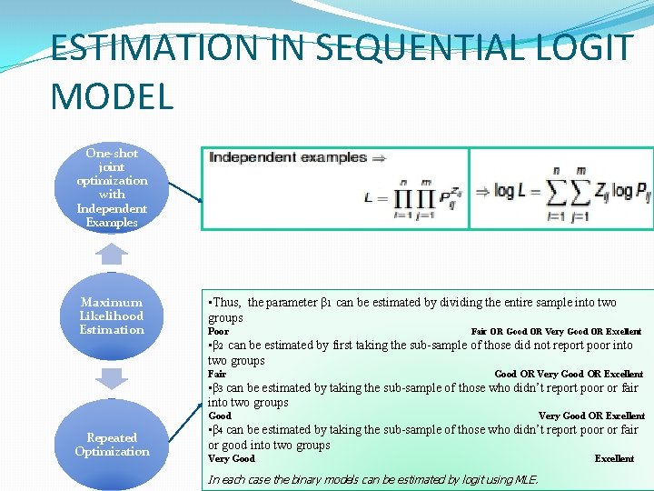
ESTIMATION IN SEQUENTIAL LOGIT MODEL One-shot joint optimization with Independent Examples Maximum Likelihood Estimation • Thus, the parameter β 1 can be estimated by dividing the entire sample into two groups Poor Fair OR Good OR Very Good OR Excellent • β 2 can be estimated by first taking the sub-sample of those did not report poor into two groups Fair Good OR Very Good OR Excellent • β 3 can be estimated by taking the sub-sample of those who didn’t report poor or fair into two groups Good Repeated Optimization Very Good OR Excellent • β 4 can be estimated by taking the sub-sample of those who didn’t report poor or fair or good into two groups Very Good In each case the binary models can be estimated by logit using MLE. Excellent

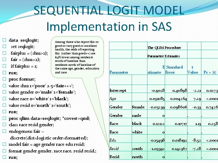
SEQUENTIAL LOGIT MODEL Implementation in SAS data seqlogit; Among those who report fair or good or very good or excellent seqlogit; health, the odds of reporting fair (rather than good++) are fairplus = (shm>1); 64% lower among residents fair = (shm=2); south of baseline than residents north of baseline of if fairplus = 1; the same age, gender, education and race. run; proc format; value shm 1='poor' 2 -5='fair+++'; value gender 0='male' 1='female'; value race 0='white' 1='black'; value resid 0='north' 1='south'; run; proc qlim data=seqlogit; *covest=qml; class race resid gender; endogenous fair ~ discrete(dist=logistic order=formatted); � model fair = age gender race edu resid; � format gender. race. resid. ; � run; � � � � The QLIM Procedure Parameter Estimates E Standard stimate Error Parameter Intercept Age Pr > |t| -0. 9028 0. 40898 -2. 21 0. 0273 0. 031085 0. 004264 7. 29 <. 0001 -0. 03239 0. 098606 -0. 33 0. 7426 Gender female Gender male 0 Race black 0. 12122 Race white 0 Edu t Value . 0. 10717 . 1. 13 . . 0. 258 . . -0. 15498 0. 018192 -8. 52 <. 0001 0. 142367 -7. 28 <. 0001 Resid south -1. 03592 Resid north 0 . . .

CONCLUSION Ordered Logit Model • Age, race, education (in terms of number of years of schooling ), and having residence in southern part of the district have a significant impact on self rated health. • Gender doesn’t have a significant impact. Sequential Logit Model • Age, education ( in terms of schooling) and having residence in southern part of the district have a significant impact on self rated health. • Gender and race don’t have significant impact.

REFERENCES • Agresti A. Categorical Data Analysis, Second edition. New York: John Wiley & Sons; 2002 • Gardiner J C. , Luo Z. Logit Models in Practice: B, C, E, G, M, N, O… SAS Institute Inc. ; 2011