Option Pricing Models I Binomial Model II BlackScholes

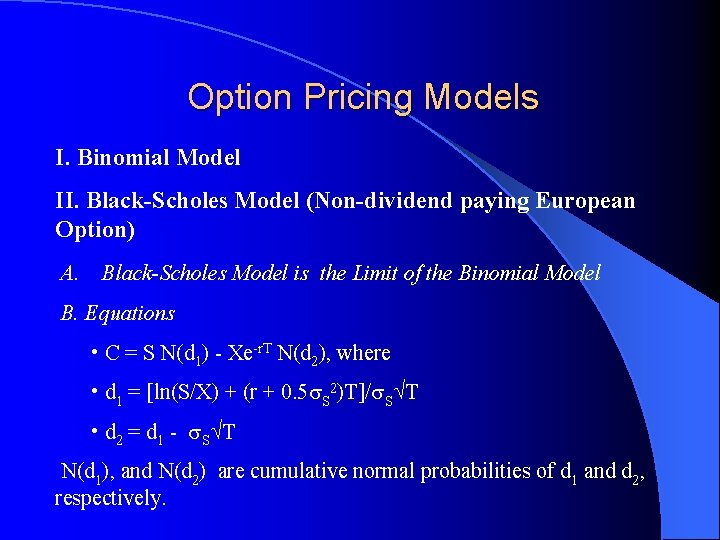
Option Pricing Models I. Binomial Model II. Black-Scholes Model (Non-dividend paying European Option) A. Black-Scholes Model is the Limit of the Binomial Model B. Equations • C = S N(d 1) - Xe-r. T N(d 2), where • d 1 = [ln(S/X) + (r + 0. 5 S 2)T]/ S T • d 2 = d 1 - S T N(d 1), and N(d 2) are cumulative normal probabilities of d 1 and d 2, respectively.

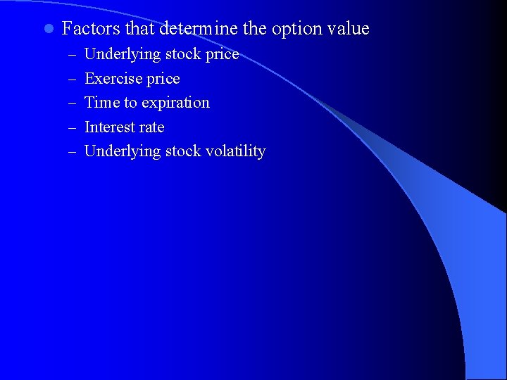
l Factors that determine the option value – Underlying stock price – Exercise price – Time to expiration – Interest rate – Underlying stock volatility

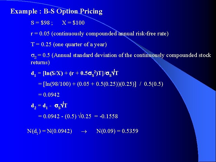
Example : B-S Option Pricing S = $98 ; X = $100 r = 0. 05 (continuously compounded annual risk-free rate) T = 0. 25 (one quarter of a year) S = 0. 5 (Annual standard deviation of the continuously compounded stock returns) d 1 = [ln(S/X) + (r + 0. 5 S 2)T]/ S T = [ln(98/100) + (0. 05 + 0. 5(0. 25))(0. 25)] / 0. 5(0. 5) = 0. 0942 d 2 = d 1 - S T = 0. 0942 - (0. 5) 0. 25 = -0. 1558 N(d 1) = N(0. 0942) N(0. 09) = 0. 5359

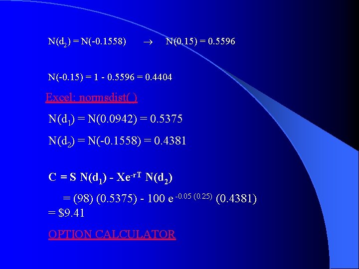
N(d 2) = N(-0. 1558) N(0. 15) = 0. 5596 N(-0. 15) = 1 - 0. 5596 = 0. 4404 Excel: normsdist( ) N(d 1) = N(0. 0942) = 0. 5375 N(d 2) = N(-0. 1558) = 0. 4381 C = S N(d 1) - Xe-r. T N(d 2) = (98) (0. 5375) - 100 e -0. 05 (0. 25) (0. 4381) = $9. 41 OPTION CALCULATOR

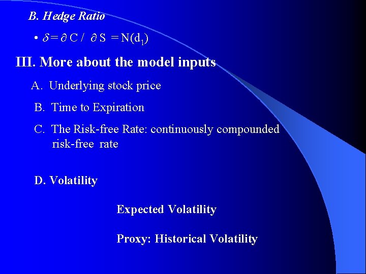
B. Hedge Ratio • = C / S = N(d 1) III. More about the model inputs A. Underlying stock price B. Time to Expiration C. The Risk-free Rate: continuously compounded risk-free rate D. Volatility Expected Volatility Proxy: Historical Volatility

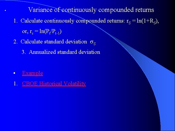
Variance of continuously compounded returns • 1. Calculate continuously compounded returns: r. S = ln(1+RS), or, rs = ln(Pt/Pt-1) 2. Calculate standard deviation S 3. Annualized standard deviation • Example 1. CBOE Historical Volatility

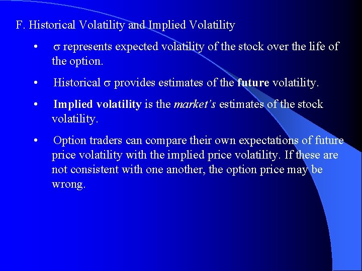
F. Historical Volatility and Implied Volatility • represents expected volatility of the stock over the life of the option. • Historical provides estimates of the future volatility. • Implied volatility is the market’s estimates of the stock volatility. • Option traders can compare their own expectations of future price volatility with the implied price volatility. If these are not consistent with one another, the option price may be wrong.

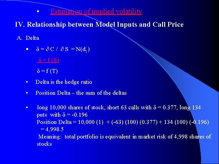
• Estimation of implied volatility IV. Relationship between Model Inputs and Call Price A. Delta = C / S = N(d 1) = f (S) = f (T) • Delta is the hedge ratio • Position Delta – the sum of the deltas • long 10, 000 shares of stock, short 63 calls with = 0. 377, long 134 puts with = -0. 196 Position Delta = 10, 000 (1) + (-63) (100) (0. 377) + 134 (100) (-0. 196) = 4, 998. 5 Meaning: total portfolio is equivalent in market risk of 4, 998 shares of stocks

l B. Gamma l = / S For stock-option hedgers, the value of measures the extent to which a change in the stock price will force a revision in the hedge ratio. = f(S) = f(T) C. Rho • = C/ i This is a liner relationship; the impact of changes in i on changes in C normally is small.

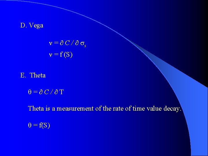
D. Vega = C / s = f (S) E. Theta = C/ T Theta is a measurement of the rate of time value decay. = f(S)

V. Put Option Pricing A. Equations • P = -S [1 -N(-d 1)] + Xe-r. T [1 -N(-d 2)], where • d 1 = [ln(S/X) + (r + 0. 5 S 2)T]/ S T • d 2 = d 1 - S T

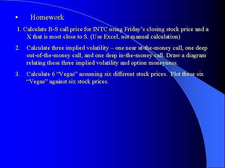
• Homework 1. Calculate B-S call price for INTC using Friday’s closing stock price and a X that is most close to S. (Use Excel, not manual calculation) 2. Calculate three implied volatility – one near at-the-money call, one deep out-of-the-money call, and one deep in-the-money call. Draw a diagram relating these three implied volatility and option moneyness. 3. Calculate 6 “Vegas” assuming six different stock prices. Plot these six “Vegas” against six stock prices.