Optimization Techniques Genetic Algorithms And other approaches for

Optimization Techniques Genetic Algorithms And other approaches for similar applications Genetic Algorithms

Optimization Techniques • • • Mathematical Programming Network Analysis Branch & Bound Genetic Algorithm Simulated Annealing Tabu Search

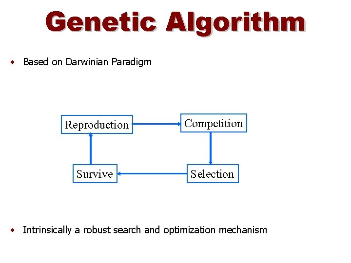
Genetic Algorithm • Based on Darwinian Paradigm Reproduction Competition Survive Selection • Intrinsically a robust search and optimization mechanism

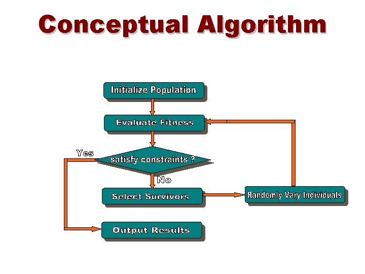
Conceptual Algorithm

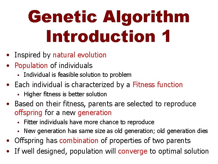
Genetic Algorithm Introduction 1 • Inspired by natural evolution • Population of individuals • Individual is feasible solution to problem • Each individual is characterized by a Fitness function • Higher fitness is better solution • Based on their fitness, parents are selected to reproduce offspring for a new generation Fitter individuals have more chance to reproduce • New generation has same size as old generation; old generation dies • • Offspring has combination of properties of two parents • If well designed, population will converge to optimal solution

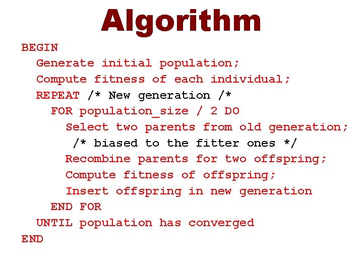
Algorithm BEGIN Generate initial population; Compute fitness of each individual; REPEAT /* New generation /* FOR population_size / 2 DO Select two parents from old generation; /* biased to the fitter ones */ Recombine parents for two offspring; Compute fitness of offspring; Insert offspring in new generation END FOR UNTIL population has converged END

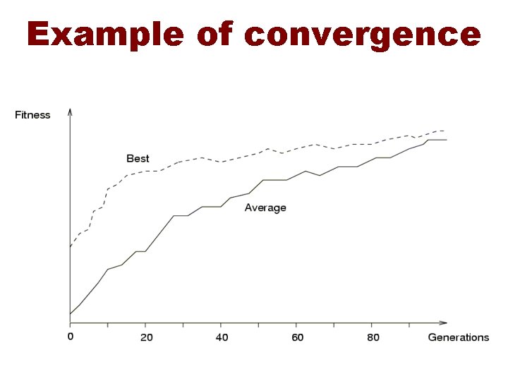
Example of convergence

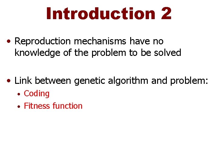
Introduction 2 • Reproduction mechanisms have no knowledge of the problem to be solved • Link between genetic algorithm and problem: Coding • Fitness function •

Basic principles 1 • Coding or Representation • String with all parameters • Fitness function • Parent selection • Reproduction Crossover • Mutation • • Convergence • When to stop

Basic principles 2 • An individual is characterized by a set of parameters: Genes • The genes are joined into a string: Chromosome • The chromosome forms the genotype • The genotype contains all information to construct an organism: the phenotype • Reproduction is a “dumb” process on the chromosome of the genotype • Fitness is measured in the real world (‘struggle for life’) of the phenotype

Coding • Parameters of the solution (genes) are concatenated to form a string (chromosome) • All kind of alphabets can be used for a chromosome (numbers, characters), but generally a binary alphabet is used • Order of genes on chromosome can be important • Generally many different codings for the parameters of a solution are possible • Good coding is probably the most important factor for the performance of a GA • In many cases many possible chromosomes do not code for feasible solutions

Genetic Algorithm • Encoding • Fitness Evaluation • Reproduction • Survivor Selection

Encoding • Design alternative individual (chromosome) • Single design choice gene • Design objectives fitness

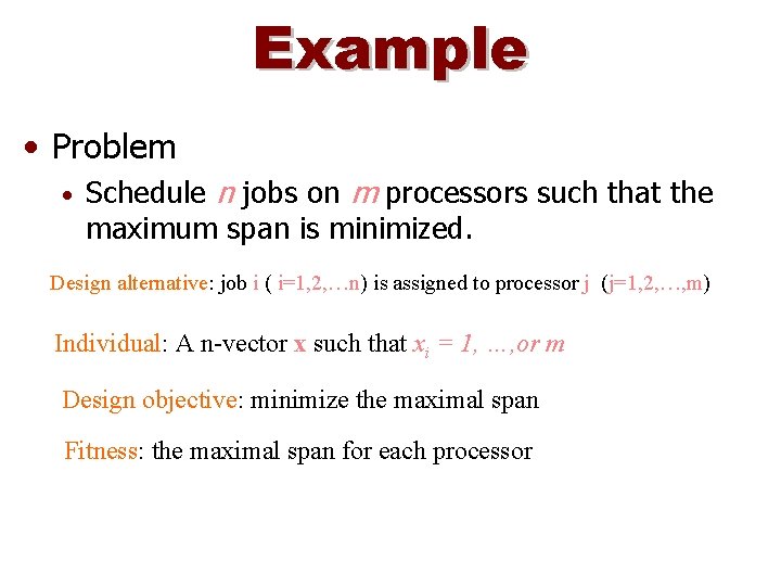
Example • Problem • Schedule n jobs on m processors such that the maximum span is minimized. Design alternative: job i ( i=1, 2, …n) is assigned to processor j (j=1, 2, …, m) Individual: A n-vector x such that xi = 1, …, or m Design objective: minimize the maximal span Fitness: the maximal span for each processor

Reproduction • Reproduction operators Crossover • Mutation •

Reproduction • Crossover Two parents produce two offspring • There is a chance that the chromosomes of the two parents are copied unmodified as offspring • There is a chance that the chromosomes of the two parents are randomly recombined (crossover) to form offspring • Generally the chance of crossover is between 0. 6 and 1. 0 • • Mutation There is a chance that a gene of a child is changed randomly • Generally the chance of mutation is low (e. g. 0. 001) •

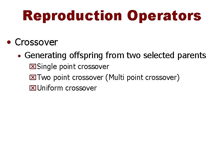
Reproduction Operators • Crossover • Generating offspring from two selected parents x. Single point crossover x. Two point crossover (Multi point crossover) x. Uniform crossover

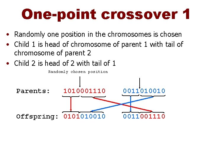
One-point crossover 1 • Randomly one position in the chromosomes is chosen • Child 1 is head of chromosome of parent 1 with tail of chromosome of parent 2 • Child 2 is head of 2 with tail of 1 Randomly chosen position Parents: 1010001110 0011010010 Offspring: 0101010010 001110

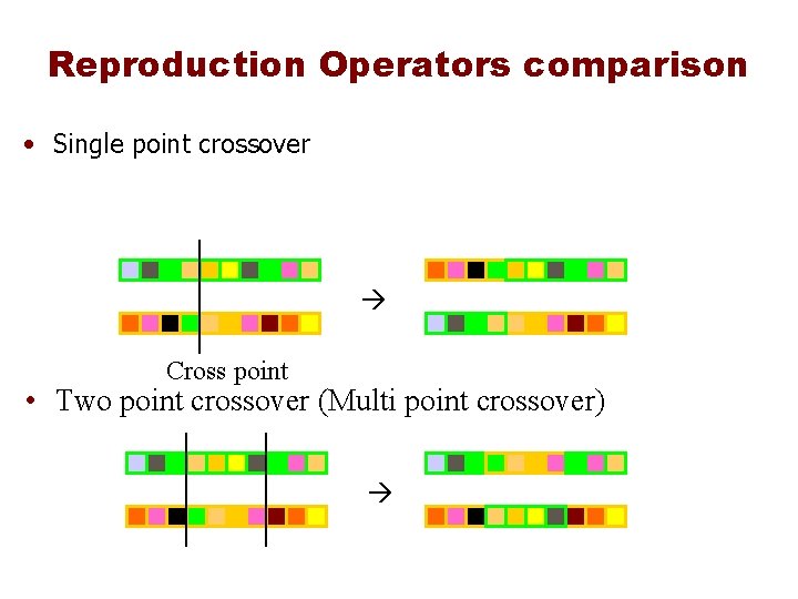
Reproduction Operators comparison • Single point crossover Cross point • Two point crossover (Multi point crossover)

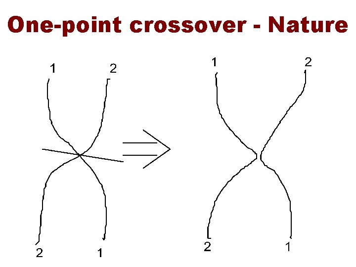
One-point crossover - Nature

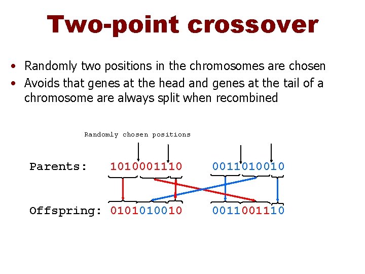
Two-point crossover • Randomly two positions in the chromosomes are chosen • Avoids that genes at the head and genes at the tail of a chromosome are always split when recombined Randomly chosen positions Parents: 1010001110 0011010010 Offspring: 0101010010 001110

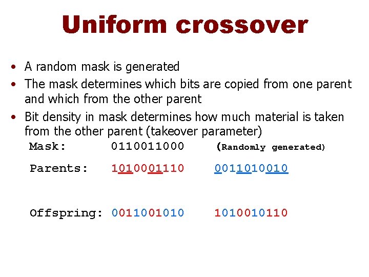
Uniform crossover • A random mask is generated • The mask determines which bits are copied from one parent and which from the other parent • Bit density in mask determines how much material is taken from the other parent (takeover parameter) Mask: 011000 (Randomly generated) Parents: 1010001110 0011010010 Offspring: 0011001010010110

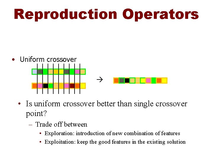
Reproduction Operators • Uniform crossover • Is uniform crossover better than single crossover point? – Trade off between • Exploration: introduction of new combination of features • Exploitation: keep the good features in the existing solution

Problems with crossover • Depending on coding, simple crossovers can have high chance to produce illegal offspring • E. g. in TSP with simple binary or path coding, most offspring will be illegal because not all cities will be in the offspring and some cities will be there more than once • Uniform crossover can often be modified to avoid this problem • E. g. in TSP with simple path coding: x. Where mask is 1, copy cities from one parent x. Where mask is 0, choose the remaining cities in the order of the other parent

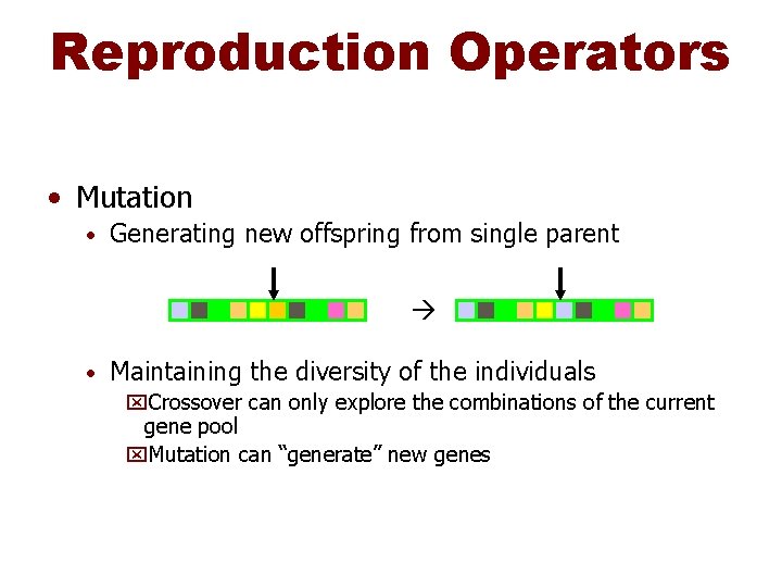
Reproduction Operators • Mutation • Generating new offspring from single parent • Maintaining the diversity of the individuals x. Crossover can only explore the combinations of the current gene pool x. Mutation can “generate” new genes

Reproduction Operators • Control parameters: probability population size, crossover/mutation Problem specific • Increase population size • x. Increase diversity and computation time for each generation • Increase crossover probability x. Increase the opportunity for recombination but also disruption of good combination • Increase mutation probability x. Closer to randomly search x. Help to introduce new gene or reintroduce the lost gene • Varies the population • Usually using crossover operators to recombine the genes to generate the new population, then using mutation operators on the new population

Parent/Survivor Selection • Strategies • Survivor selection x. Always keep the best one x. Elitist: deletion of the K worst x. Probability selection : inverse to their fitness x. Etc.

Parent/Survivor Selection • Too strong fitness selection bias can lead to suboptimal solution • Too little fitness bias selection results in unfocused and meandering search

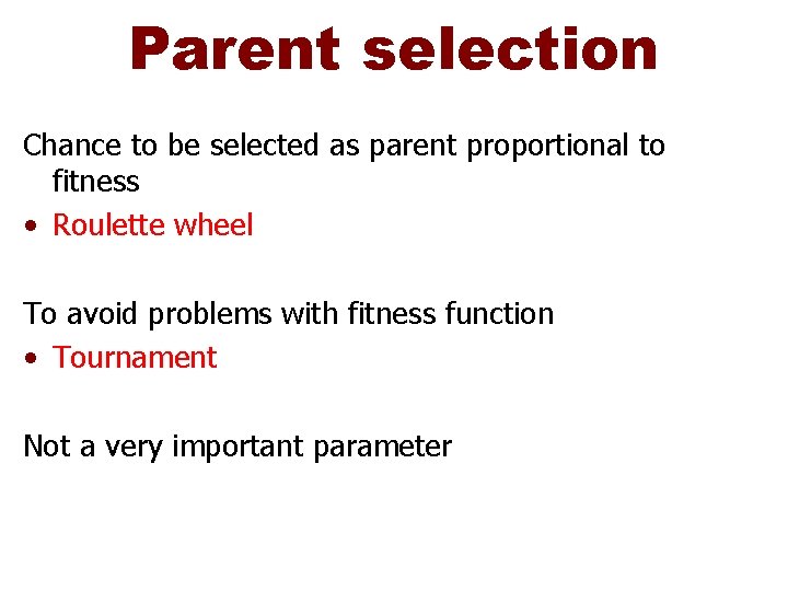
Parent selection Chance to be selected as parent proportional to fitness • Roulette wheel To avoid problems with fitness function • Tournament Not a very important parameter

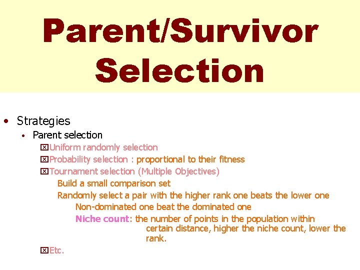
Parent/Survivor Selection • Strategies • Parent selection x. Uniform randomly selection x. Probability selection : proportional to their fitness x. Tournament selection (Multiple Objectives) Build a small comparison set Randomly select a pair with the higher rank one beats the lower one Non-dominated one beat the dominated one Niche count: the number of points in the population within certain distance, higher the niche count, lower the rank. x. Etc.

Others • • Global Optimal Parameter Tuning Parallelism Random number generators

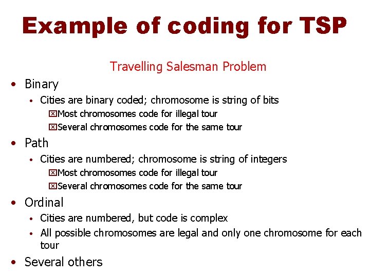
Example of coding for TSP Travelling Salesman Problem • Binary • Cities are binary coded; chromosome is string of bits x. Most chromosomes code for illegal tour x. Several chromosomes code for the same tour • Path • Cities are numbered; chromosome is string of integers x. Most chromosomes code for illegal tour x. Several chromosomes code for the same tour • Ordinal Cities are numbered, but code is complex • All possible chromosomes are legal and only one chromosome for each tour • • Several others

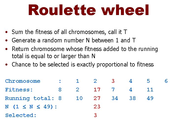
Roulette wheel • Sum the fitness of all chromosomes, call it T • Generate a random number N between 1 and T • Return chromosome whose fitness added to the running total is equal to or larger than N • Chance to be selected is exactly proportional to fitness Chromosome : Fitness: 8 Running total: 8 N (1 N 49): Selected: 1 2 10 2 17 27 23 3 3 7 34 4 4 38 5 11 49 6

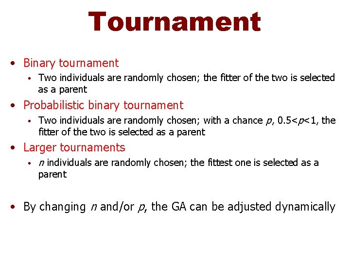
Tournament • Binary tournament • Two individuals are randomly chosen; the fitter of the two is selected as a parent • Probabilistic binary tournament • Two individuals are randomly chosen; with a chance p, 0. 5<p<1, the fitter of the two is selected as a parent • Larger tournaments • n individuals are randomly chosen; the fittest one is selected as a parent • By changing n and/or p, the GA can be adjusted dynamically

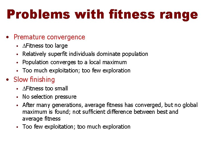
Problems with fitness range • Premature convergence Fitness too large • Relatively superfit individuals dominate population • Population converges to a local maximum • Too much exploitation; too few exploration • • Slow finishing Fitness too small • No selection pressure • After many generations, average fitness has converged, but no global maximum is found; not sufficient difference between best and average fitness • Too few exploitation; too much exploration •

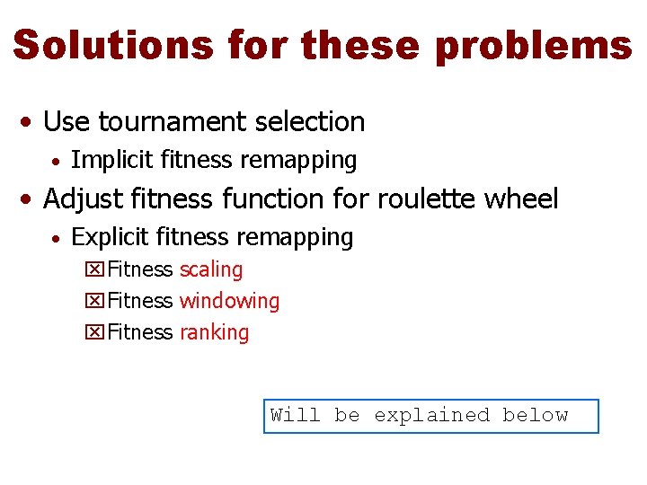
Solutions for these problems • Use tournament selection • Implicit fitness remapping • Adjust fitness function for roulette wheel • Explicit fitness remapping x. Fitness scaling x. Fitness windowing x. Fitness ranking Will be explained below

Fitness Function Purpose • Parent selection • Measure for convergence • For Steady state: Selection of individuals to die • Should reflect the value of the chromosome in some “real” way • Next to coding the most critical part of a GA

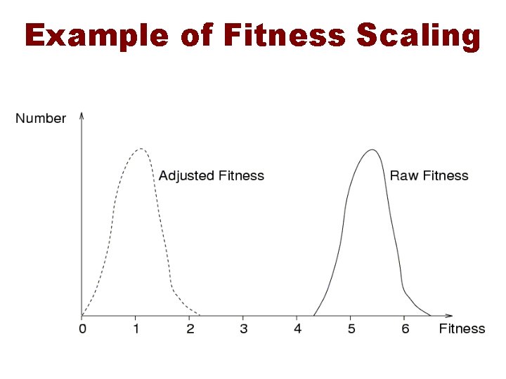
Fitness scaling • Fitness values are scaled by subtraction and division so that worst value is close to 0 and the best value is close to a certain value, typically 2 Chance for the most fit individual is 2 times the average • Chance for the least fit individual is close to 0 • • Problems when the original maximum is very extreme (super -fit) or when the original minimum is very extreme (superunfit) • Can be solved by defining a minimum and/or a maximum value for the fitness

Example of Fitness Scaling

Fitness windowing • Same as window scaling, except the amount subtracted is the minimum observed in the n previous generations, with n e. g. 10 • Same problems as with scaling

Fitness ranking • Individuals are numbered in order of increasing fitness • The rank in this order is the adjusted fitness • Starting number and increment can be chosen in several ways and influence the results • No problems with super-fit or super-unfit • Often superior to scaling and windowing

Fitness Evaluation • A key component in GA • Time/quality trade off • Multi-criterion fitness

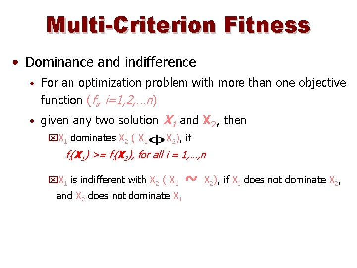
Multi-Criterion Fitness • Dominance and indifference • For an optimization problem with more than one objective function (fi, i=1, 2, …n) • given any two solution X 1 and X 2, then x. X 1 dominates X 2 ( X 1 X 2), if fi(X 1) >= fi(X 2), for all i = 1, …, n x. X 1 is indifferent with X 2 ( X 1 and X 2 does not dominate X 1 ~ X 2), if X 1 does not dominate X 2,

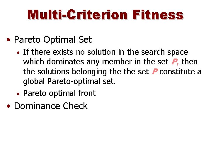
Multi-Criterion Fitness • Pareto Optimal Set If there exists no solution in the search space which dominates any member in the set P, then the solutions belonging the set P constitute a global Pareto-optimal set. • Pareto optimal front • • Dominance Check

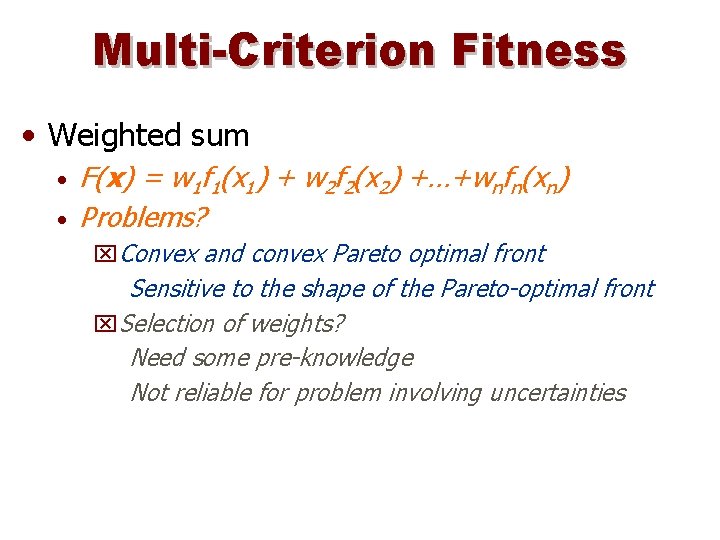
Multi-Criterion Fitness • Weighted sum • • F(x) = w 1 f 1(x 1) + w 2 f 2(x 2) +…+wnfn(xn) Problems? x. Convex and convex Pareto optimal front Sensitive to the shape of the Pareto-optimal front x. Selection of weights? Need some pre-knowledge Not reliable for problem involving uncertainties

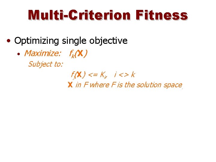
Multi-Criterion Fitness • Optimizing single objective • Maximize: fk(X) Subject to: fj(X) <= Ki, i <> k X in F where F is the solution space.

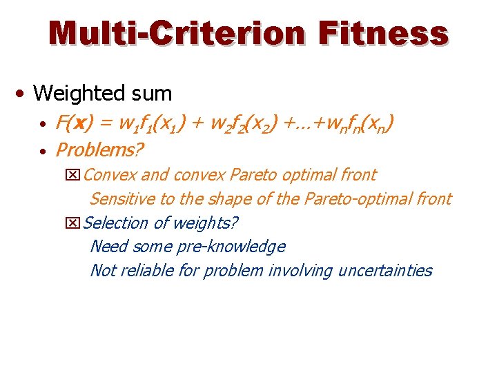
Multi-Criterion Fitness • Weighted sum • • F(x) = w 1 f 1(x 1) + w 2 f 2(x 2) +…+wnfn(xn) Problems? x. Convex and convex Pareto optimal front Sensitive to the shape of the Pareto-optimal front x. Selection of weights? Need some pre-knowledge Not reliable for problem involving uncertainties

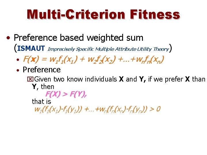
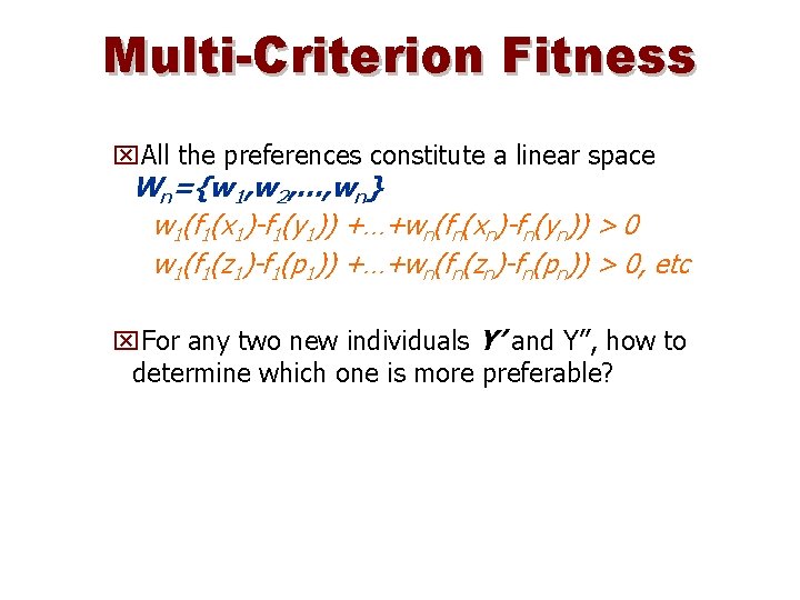
Multi-Criterion Fitness • Preference based weighted sum (ISMAUT Imprecisely Specific Multiple Attribute Utility Theory) • • F(x) = w 1 f 1(x 1) + w 2 f 2(x 2) +…+wnfn(xn) Preference x. Given two know individuals X and Y, if we prefer X than Y, then F(X) > F(Y), that is w 1(f 1(x 1)-f 1(y 1)) +…+wn(fn(xn)-fn(yn)) > 0

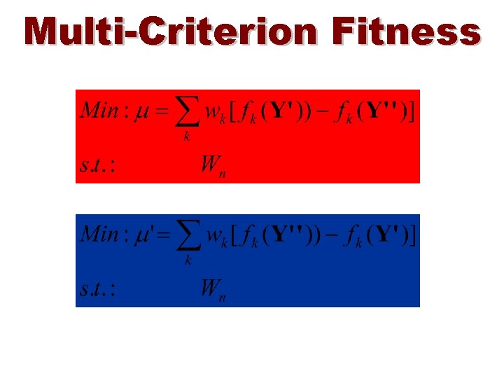
Multi-Criterion Fitness x. All the preferences constitute a linear space Wn={w 1, w 2, …, wn} w 1(f 1(x 1)-f 1(y 1)) +…+wn(fn(xn)-fn(yn)) > 0 w 1(f 1(z 1)-f 1(p 1)) +…+wn(fn(zn)-fn(pn)) > 0, etc x. For any two new individuals Y’ and Y’’, how to determine which one is more preferable?

Multi-Criterion Fitness

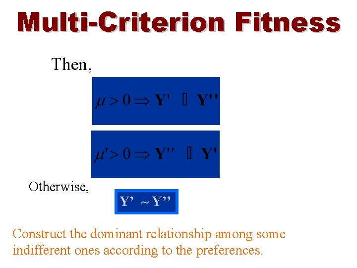
Multi-Criterion Fitness Then, Otherwise, Y’ ~ Y’’ Construct the dominant relationship among some indifferent ones according to the preferences.

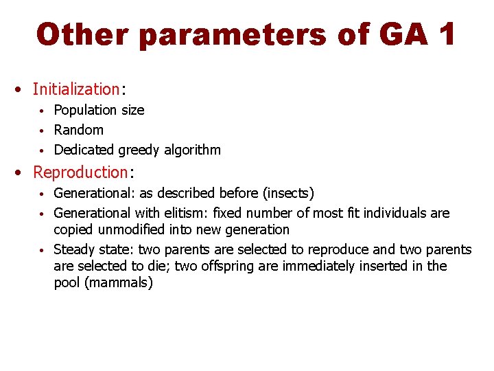
Other parameters of GA 1 • Initialization: Population size • Random • Dedicated greedy algorithm • • Reproduction: Generational: as described before (insects) • Generational with elitism: fixed number of most fit individuals are copied unmodified into new generation • Steady state: two parents are selected to reproduce and two parents are selected to die; two offspring are immediately inserted in the pool (mammals) •

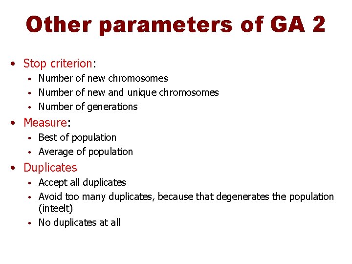
Other parameters of GA 2 • Stop criterion: Number of new chromosomes • Number of new and unique chromosomes • Number of generations • • Measure: Best of population • Average of population • • Duplicates Accept all duplicates • Avoid too many duplicates, because that degenerates the population (inteelt) • No duplicates at all •

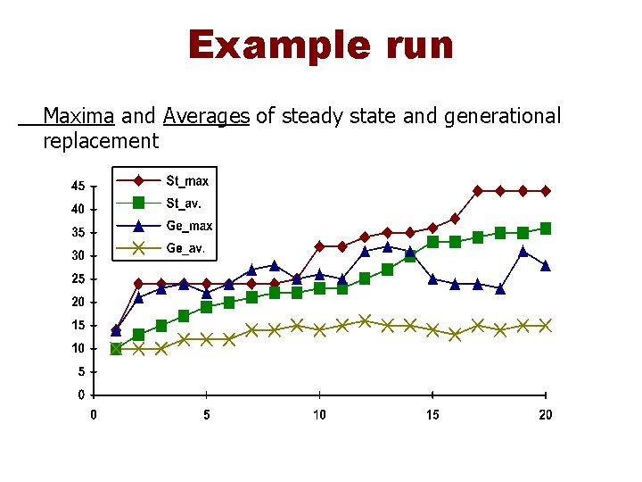
Example run Maxima and Averages of steady state and generational replacement

Simulated Annealing • What • Exploits an analogy between the annealing process and the search for the optimum in a more general system.

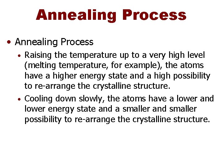
Annealing Process • Annealing Process Raising the temperature up to a very high level (melting temperature, for example), the atoms have a higher energy state and a high possibility to re-arrange the crystalline structure. • Cooling down slowly, the atoms have a lower and lower energy state and a smaller and smaller possibility to re-arrange the crystalline structure. •

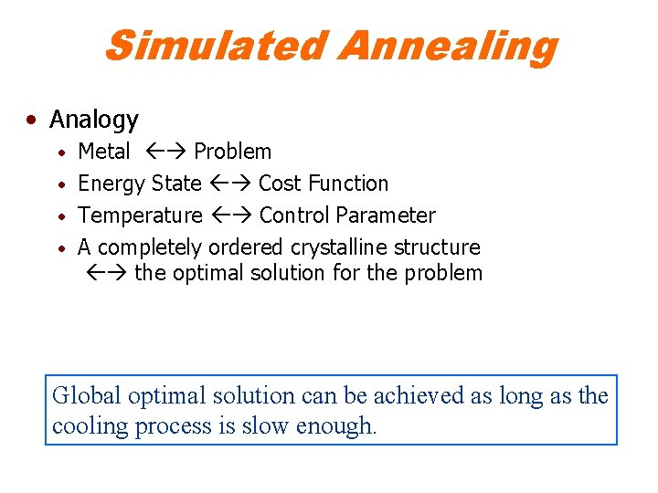
Simulated Annealing • Analogy Metal Problem • Energy State Cost Function • Temperature Control Parameter • A completely ordered crystalline structure the optimal solution for the problem • Global optimal solution can be achieved as long as the cooling process is slow enough.

Metropolis Loop • The essential characteristic of simulated annealing • Determining how to randomly explore new solution, reject or accept the new solution at a constant temperature T. • Finished until equilibrium is achieved.

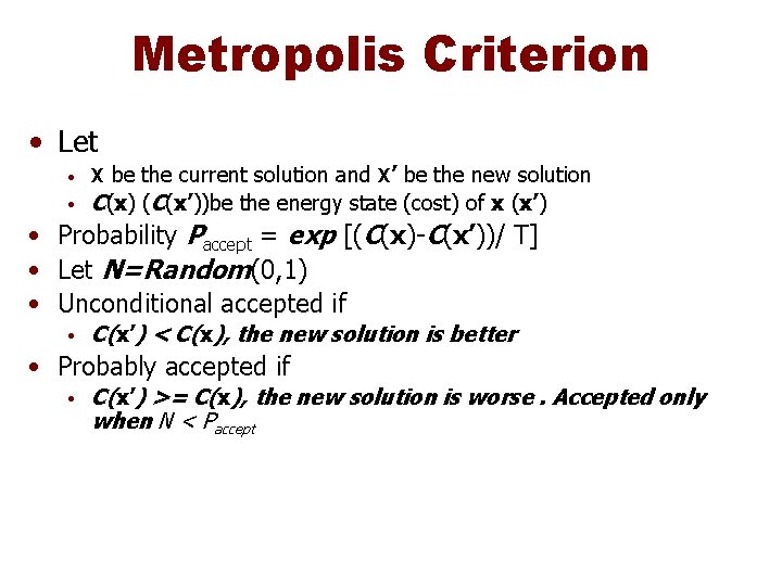
Metropolis Criterion • Let • X be the current solution and X’ be the new solution • C(x) (C(x’))be the energy state (cost) of x (x’) • Probability Paccept = exp [(C(x)-C(x’))/ T] • Let N=Random(0, 1) • Unconditional accepted if • C(x’) < C(x), the new solution is better • Probably accepted if • C(x’) >= C(x), the new solution is worse. Accepted only when N < Paccept

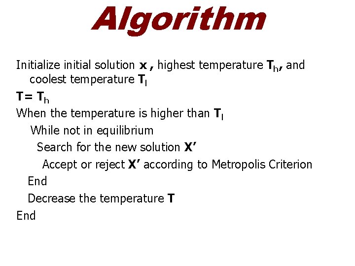
Algorithm Initialize initial solution x , highest temperature Th, and coolest temperature Tl T= Th When the temperature is higher than Tl While not in equilibrium Search for the new solution X’ Accept or reject X’ according to Metropolis Criterion End Decrease the temperature T End

Simulated Annealing • Definition of solution • Search mechanism, i. e. the definition of a neighborhood • Cost-function

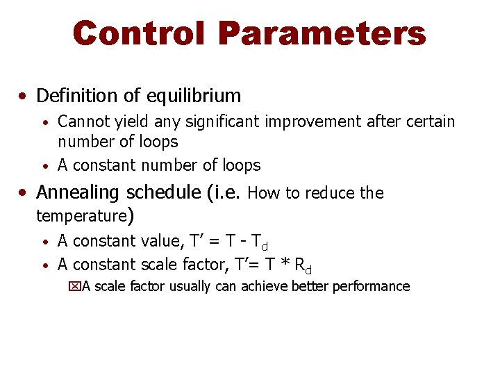
Control Parameters • Definition of equilibrium Cannot yield any significant improvement after certain number of loops • A constant number of loops • • Annealing schedule (i. e. How to reduce the temperature) A constant value, T’ = T - Td • A constant scale factor, T’= T * Rd • x. A scale factor usually can achieve better performance

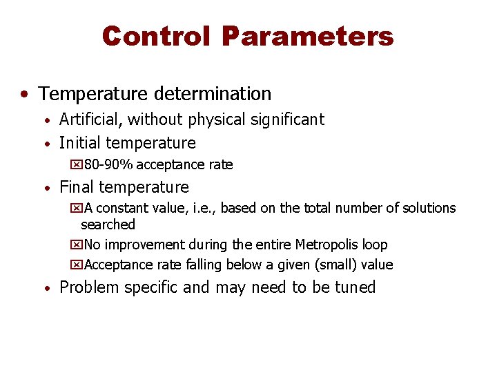
Control Parameters • Temperature determination Artificial, without physical significant • Initial temperature • x 80 -90% acceptance rate • Final temperature x. A constant value, i. e. , based on the total number of solutions searched x. No improvement during the entire Metropolis loop x. Acceptance rate falling below a given (small) value • Problem specific and may need to be tuned

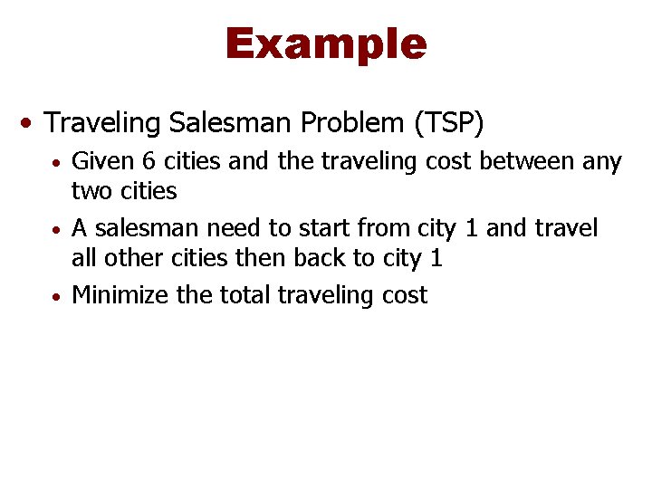
Example • Traveling Salesman Problem (TSP) Given 6 cities and the traveling cost between any two cities • A salesman need to start from city 1 and travel all other cities then back to city 1 • Minimize the total traveling cost •

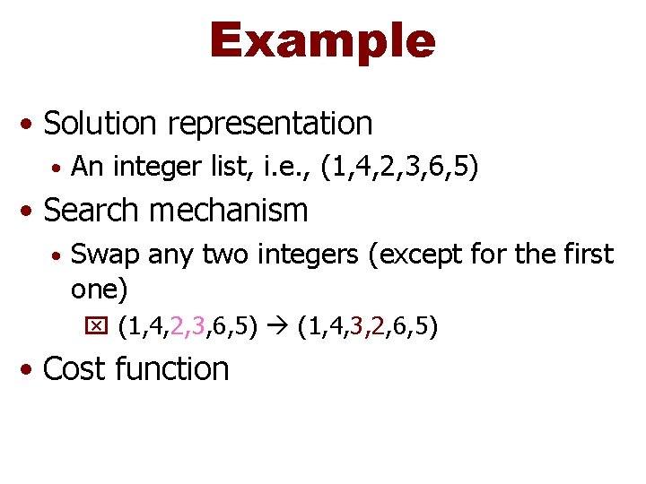
Example • Solution representation • An integer list, i. e. , (1, 4, 2, 3, 6, 5) • Search mechanism • Swap any two integers (except for the first one) x (1, 4, 2, 3, 6, 5) (1, 4, 3, 2, 6, 5) • Cost function

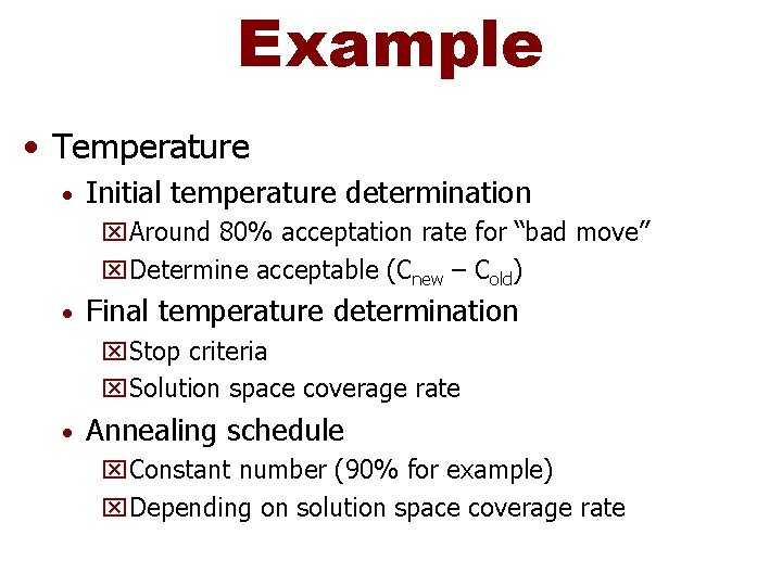
Example • Temperature • Initial temperature determination x. Around 80% acceptation rate for “bad move” x. Determine acceptable (Cnew – Cold) • Final temperature determination x. Stop criteria x. Solution space coverage rate • Annealing schedule x. Constant number (90% for example) x. Depending on solution space coverage rate

Others • Global optimal is possible, but near optimal is practical • Parameter Tuning – Aarts, E. and Korst, J. (1989). Simulated Annealing and Boltzmann Machines. John Wiley & Sons. • Not easy for parallel implementation • Randomly generator

Optimization Techniques • • • Mathematical Programming Network Analysis Branch & Bound Genetic Algorithm Simulated Annealing Tabu Search

Tabu Search • What • Neighborhood search + memory x. Neighborhood search x. Memory Record the search history Forbid cycling search

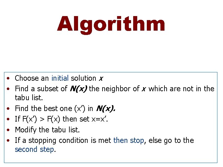
Algorithm • Choose an initial solution X • Find a subset of N(x) the neighbor of X which are not in the tabu list. • Find the best one (x’) in N(x). • If F(x’) > F(x) then set x=x’. • Modify the tabu list. • If a stopping condition is met then stop, else go to the second step.

Effective Tabu Search • Effective Modeling Neighborhood structure • Objective function (fitness or cost) • x. Example Graph coloring problem: Find the minimum number of colors needed such that no two connected nodes share the same color. • Aspiration criteria • The criteria for overruling the tabu constraints and differentiating the preference of among the neighbors

Effective Tabu Search • Effective Computing • “Move” may be easier to be stored and computed than a completed solution xmove: the process of constructing of x’ from x • Computing and storing the fitness difference may be easier than that of the fitness function.

Effective Tabu Search • Effective Memory Use • Variable tabu list size x. For a constant size tabu list Too long: deteriorate the search results Too short: cannot effectively prevent from cycling • Intensification of the search x. Decrease the tabu list size • Diversification of the search x. Increase the tabu list size x. Penalize the frequent move or unsatisfied constraints

Example • A hybrid approach for graph coloring problem • R. Dorne and J. K. Hao, A New Genetic Local Search Algorithm for Graph Coloring, 1998

Problem • Given an undirected graph G=(V, E) • • V={v 1, v 2, …, vn} E={eij} • Determine a partition of V in a minimum number of color classes C 1, C 2, …, Ck such that for each edge eij, vi and vj are not in the same color class. • NP-hard

General Approach • Transform an optimization problem into a decision problem • Genetic Algorithm + Tabu Search Meaningful crossover • Using Tabu search for efficient local search •

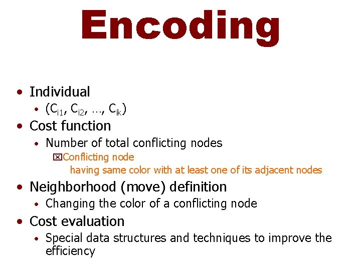
Encoding • Individual • (Ci 1, Ci 2, …, Cik) • Cost function • Number of total conflicting nodes x. Conflicting node having same color with at least one of its adjacent nodes • Neighborhood (move) definition • Changing the color of a conflicting node • Cost evaluation • Special data structures and techniques to improve the efficiency

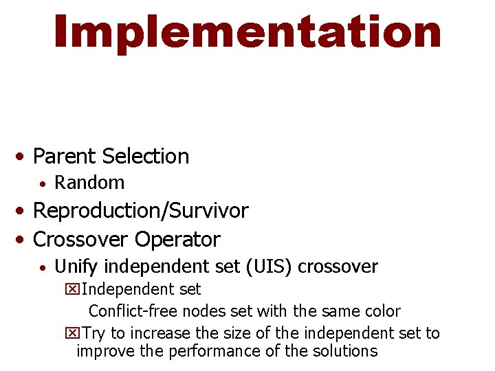
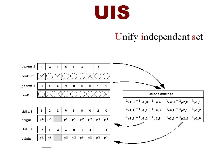
Implementation • Parent Selection • Random • Reproduction/Survivor • Crossover Operator • Unify independent set (UIS) crossover x. Independent set Conflict-free nodes set with the same color x. Try to increase the size of the independent set to improve the performance of the solutions

UIS Unify independent set

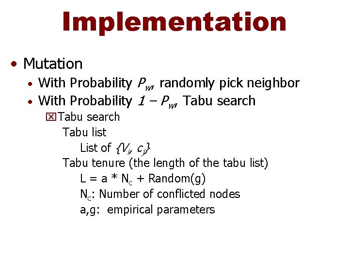
Implementation • Mutation With Probability Pw, randomly pick neighbor • With Probability 1 – Pw, Tabu search • x. Tabu search Tabu list List of {Vi, cj} Tabu tenure (the length of the tabu list) L = a * Nc + Random(g) Nc: Number of conflicted nodes a, g: empirical parameters

Summary • Neighbor Search • TS prevent being trapped in the local minimum with tabu list • TS directs the selection of neighbor • TS cannot guarantee the optimal result • Sequential • Adaptive

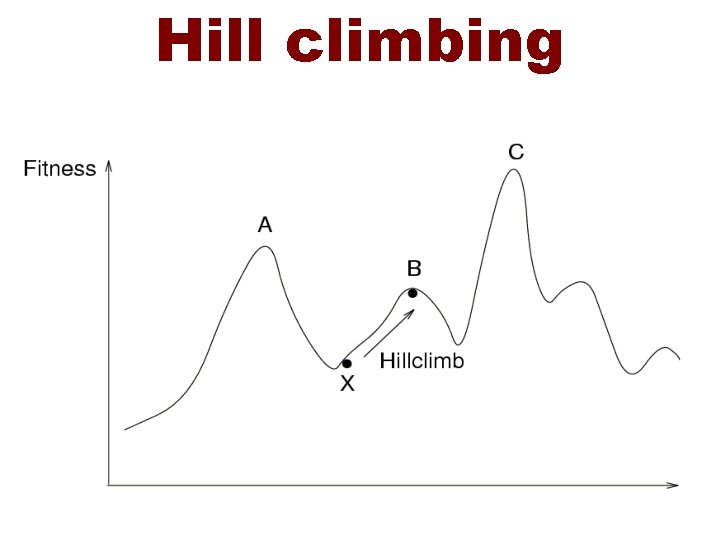
Hill climbing

sources Jaap Hofstede, Beasly, Bull, Martin Version 2, October 2000 Department of Computer Science & Engineering University of South Carolina Spring, 2002 Genetic Algorithms