Optimization in Electrical Engineering Professor David Thiel Centre

Optimization in Electrical Engineering Professor David Thiel Centre for Wireless Monitoring and Applications Griffith University, Brisbane Australia 1

My Interest? • Interpretation of geophysical data when there are more knowns than unknowns. • Optimizing antennas for maximum gain and minimal materials. • Using lumped impedance elements to achieve dual frequency operations. • Working with improved performance of switched parasitic antennas 2

Purpose • To make attendees familiar with the process of optimization in electrical engineering. • To introduce the basic elements of an optimisation routine including: – – – Initial parameters Forward modelling Cost function Guided parameter refinement Program termination 3

Why Optimisation? It is no longer acceptable to submit a new design to a journal or conference without logical support for the idea. One can gain support for the new design using theory or optimisation. 4

Workshop Strategy • • • I will not include many equations. Generally these equations are relatively simple, can be found in books, and can be derived using simple geometry. In some places the equations can’t be avoided and so have been included. Optimisation is usually conducted in multidimensional space and so it quite difficult to visualize. We will use a 2 D model so we can visualize! 5

Optimization applications • Standard curve fitting procedures require more data points than the number of unknowns to find. • For example, linear correlation defines the slope and the intercept from a set of data points. (see the Research Methods workshop) • Optimization allows the determination of more unknowns that there are data points. 6

Optimization is curve fitting/pattern recognition • The optimization routine generates improved “guesses” to minimize the cost function – for curve fitting, the cost function is the RMS error. • In optimization, the Cost function is minimized – the RMS error is minimized. 7

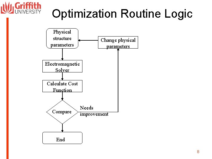
Optimization Routine Logic Physical structure parameters Change physical parameters Electromagnetic Solver Calculate Cost Function Compare Needs improvement End 8

Physical Structure • Assume we wish to optimize n parameters in the physical structure. All other parameters remain fixed. • Set the limits on each parameter (maxima and minima) • Set minimum step size (manufacturing tolerances) • Guess the first structure (by random selection? ). 9

Electromagnetic Solver • Open boundary (eg Method of Moments) or closed boundary (eg FEM, FDTD) • Set segment/pixel/voxel size • Pre-processing requirements? • Post-processing requirements? (eg time to frequency domain? ) • This is often the rate determining step in an optimization routine. Open boundary methods are usually more efficient compared to closed boundary methods. 10

Define the Cost Function • What are the most important parameters in the final design? • For antennas it might be: – – – – Gain Front to back ratio Efficiency Input impedance Weight Wind resistance Environmental impact 11

Define the Cost Function • The parameters in the cost function can be weighted to give the correct emphasis in the final outcome. • The optimization routine is designed to minimize the cost function. • It is the inverse of a “Figure of merit”. 12

Compare • Every updated cost function (often called the next generation or the next iteration) is compared to the last. • If the design has improved (lower cost function value), continue changing the design in the same direction. • If the design is worse (higher cost function value), change the design in a different direction. • If no significant change, then terminate the routine. 13

Change the physical structure • There are many methods of doing this. Some are guided and others are unguided (random) • We will discuss: – – Sequential uniform sampling The Monte Carlo Method The Simplex Method The Method of Steepest Descent (the Gradient Method) – The Genetic Algorithm – Simulated Annealing 14

Method 1 Sequential Uniform Sampling (SUS) 15

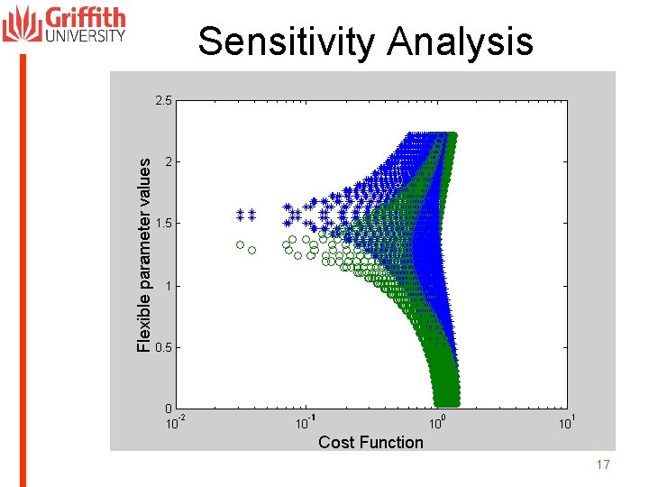
Sequential uniform sampling • Calculate every possible combination of every parameter (n) through every increment specified. • Chose the design with the lowest value of the cost function. • A plot of the data will give an indication of the robustness of the solution. • The best solution can be improved by using finer increments and smaller range values. 16

Sensitivity Analysis 17

SUS: Comments • The best solution can be improved by using finer increments and smaller range values. • The results give an idea of which design parameters are critical and which are not so critical. 18

SUS: Advantages • The cost function is never trapped in a local minima. • There is no random element. There is no need to repeat the same trial as you will get the same answer. 19

SUS: Problems • This is an unguided optimization process. • This is extremely computationally intensive. 20

Method 2 Monte Carlo (MC) (Random Sampling) 21

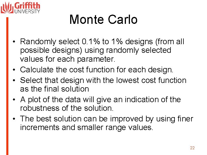
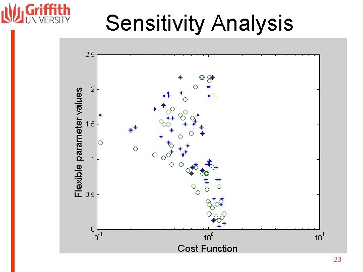
Monte Carlo • Randomly select 0. 1% to 1% designs (from all possible designs) using randomly selected values for each parameter. • Calculate the cost function for each design. • Select that design with the lowest cost function as the final solution • A plot of the data will give an indication of the robustness of the solution. • The best solution can be improved by using finer increments and smaller range values. 22

Sensitivity Analysis 23

Monte Carlo: Comments • The best solution can be improved by using finer increments and smaller range values. 24

Monte Carlo: Advantages • This is less computationally intensive compared to SUS. • The solution is not trapped in a local minimum. 25

Monte Carlo: Problems • It is more computationally intensive compared to many guided optimisation methods. • It is likely that every run will result in a different solution. You never know if/when you have reached the best solution. 26

Method 3 The Simplex Method 27

Simplex Method • Randomly select the first design and calculate the cost function. • Increment one parameter and recalculate the cost function. • Do this for every parameter in the design. • These cost function values form a “simplex” in n dimensional space. 28

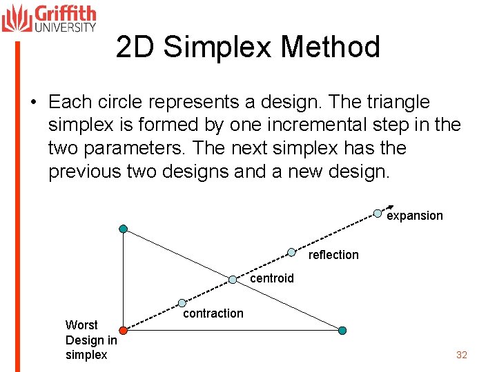
Simplex Method • Calculate the centre of mass (centroid) of the simplex. • Draw a line from the high valued cost function, through the centre of mass. • The new design lies along this line and is the mirrored point through the opposite surface (n-1 dimensions) defined by the other designs – called reflection. 29

Simplex Method • If the cost function is lower than the highest cost function, replace this new point in the simplex. • If the cost function is much lower than the highest cost function, increase the step size and replace this new point in the simplex – called expansion. • Repeat the calculations until no further improvement is gained. 30

Simplex Method • If the cost function is higher than the highest cost function, reduce the step size and replace this new point in the simplex – called contraction. • Repeat the calculations until no further improvement is gained by any of these three operations. 31

2 D Simplex Method • Each circle represents a design. The triangle simplex is formed by one incremental step in the two parameters. The next simplex has the previous two designs and a new design. expansion reflection centroid Worst Design in simplex contraction 32

Simplex Method: Comments • To reduce falling into a local minima, repeat the algorithm a number of times with a new randomly selected design. 33

Simplex Method: Advantages • It is a guided algorithm – the cost function always decreases until the final solution is reached. 34

Simplex Method: Problems • This method is prone to getting trapped in “local” cost function minima. Continuing with the algorithm does not improve the solution. • At a n D saddle point of the cost function surface, the simplex routine may simply repeat every second iteration. • The method is not very efficient in locating the minimum cost function value. 35

Method 4 The Gradient Method (Method of Steepest Descent) 36

Gradient Method • Calculate the simplex. • Calculate the vector gradient of the cost function and use this value to locate the new design point. • Repeat until no improvement is observed. • The “distance” of the step along the line of maximum descent is related to absolute value of the gradient. 37

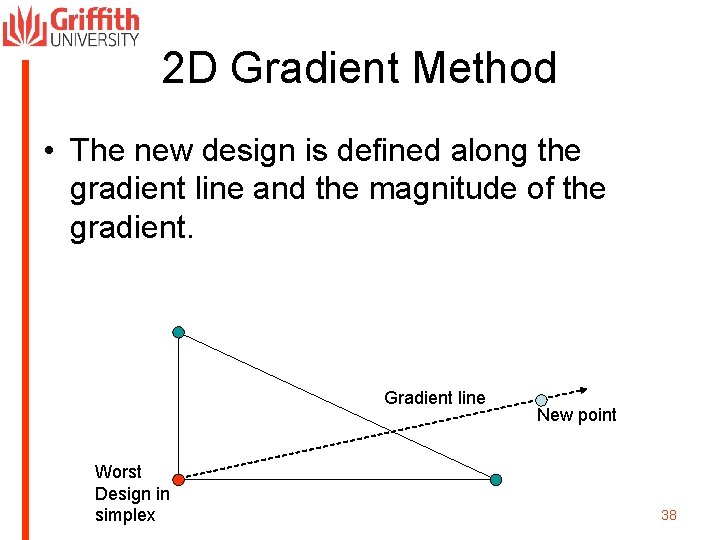
2 D Gradient Method • The new design is defined along the gradient line and the magnitude of the gradient. Gradient line Worst Design in simplex New point 38

Gradient Method: Comments • To reduce falling into a local minima, repeat the algorithm a number of times with a new randomly selected design. 39

Gradient Method: Advantages • This is more efficient compared to the simplex method as all cost function values in the simplex are used to calculate the direction. This means all parameters are changed at every iteration. 40

Gradient Method: Problems • It can still be trapped in local minima. • It can still be trapped in a saddle point. 41

Method 5 The Genetic Algorithm (GA) (Modelled on Darwin’s theory of natural selection Survival of the fittest) 42

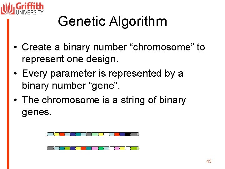
Genetic Algorithm • Create a binary number “chromosome” to represent one design. • Every parameter is represented by a binary number “gene”. • The chromosome is a string of binary genes. 43

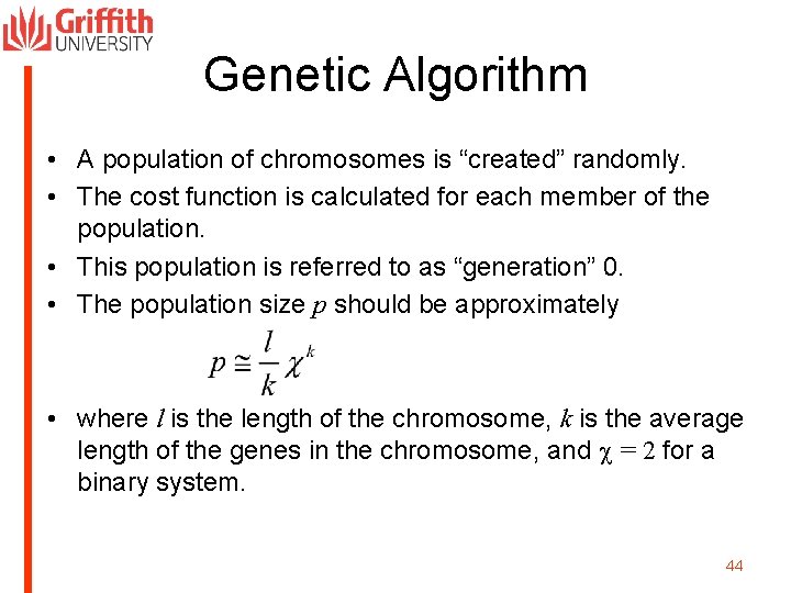
Genetic Algorithm • A population of chromosomes is “created” randomly. • The cost function is calculated for each member of the population. • This population is referred to as “generation” 0. • The population size p should be approximately • where l is the length of the chromosome, k is the average length of the genes in the chromosome, and c = 2 for a binary system. 44

Genetic Algorithm • Generation 1 is formed from generation 0 using genetic processes of “death”, “mutation”, “creation”, “cloning” and “crossover/mating”. • Every generation should have the same population size p. 45

Death • In the “survival of the fittest”, those chromosomes with a very poor cost function are removed from the population. • This is usually half the population. • The following processes are used to replenish the population. 46

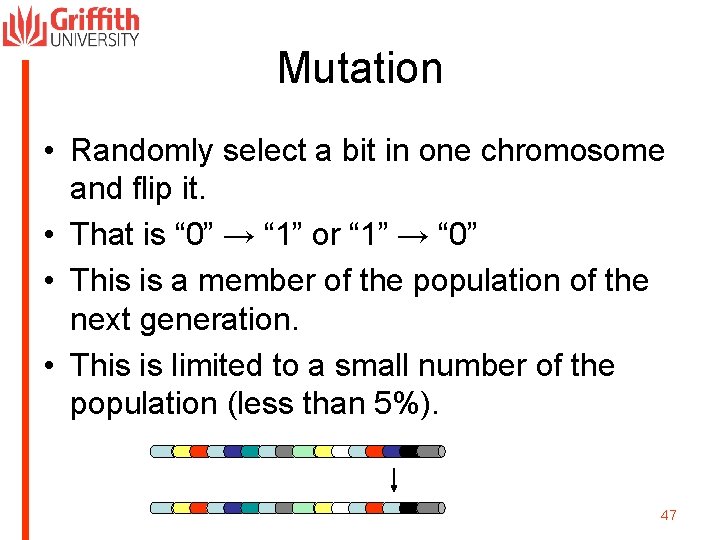
Mutation • Randomly select a bit in one chromosome and flip it. • That is “ 0” → “ 1” or “ 1” → “ 0” • This is a member of the population of the next generation. • This is limited to a small number of the population (less than 5%). 47

Cloning • Copy one chromosome (usually with a low cost function) into the next generation. • This is often a large portion of the population (up to 50%) 48

Creation • Randomly generate another chromosome and place into the population of the new generation. • This is limited to a small number of the population (less than 5%). 49

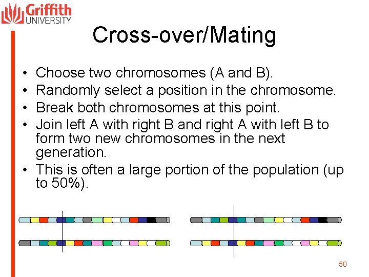
Cross-over/Mating • • Choose two chromosomes (A and B). Randomly select a position in the chromosome. Break both chromosomes at this point. Join left A with right B and right A with left B to form two new chromosomes in the next generation. • This is often a large portion of the population (up to 50%). 50

Genetic Algorithm • Successive generations are produced and cost functions calculated. • When the smallest cost function in the population does not change after many iterations, the routine is terminated. 51

Genetic Algorithm: Comments • A plot of the cost function data set will give an indication of the robustness of the solution. • These are random processes so the algorithm must be repeated a number of times. The convergence is never the same. • The chromosomes need to be unpacked for the solver. 52

GA: Problems • This method is computationally intensive for many problems. • The final result might not be the best design. 53

GA: Advantages • It is possible to keep multiple “good” designs in the population. • The routine can escape from local minima due to the random processes (creation, mutation and mating). 54

Method 6 Simulated Annealing (Modelled on the annealing of steel for sword making) 55

Simulated Annealing • Randomly select the first design parameters and calculate the cost function C 1. • Randomly select one parameter and increment/decrement to obtain the next design and calculate the new cost function C 2. 56

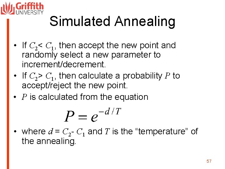
Simulated Annealing • If C 2< C 1, then accept the new point and randomly select a new parameter to increment/decrement. • If C 2> C 1, then calculate a probability P to accept/reject the new point. • P is calculated from the equation • where d = C 2 - C 1 and T is the “temperature” of the annealing. 57

Simulated Annealing • Generate a new number x randomly, where • 0 < x <1. • If P/x > 1, then accept new design and decrement T. • If P/x < 1, then reject new design and chose a different parameter/direction to change. • As algorithm progresses, T decreases to the point where the probability of accepting a change in the wrong direction is highly unlikely. 58

Simulated Annealing • When T = 0, the design is “quenched” and no further changes in the wrong direction are allowed. (T can not be less than 0). • The routine terminates when no more changes are allowed. 59

Simulated Annealing: Comments • There is a finite probability that a transition from a local minimum is possible, but only when the temperature is high enough. • Very dependent on the “best” selection of the incremental change in temperature. – If T decreases too rapidly, there is a higher probability of getting trapped in a local minima. – If T decreases too slowly, convergence is too slow. 60

Simulated Annealing: Strengths • There is a finite probability that a transition from a local minimum is possible, but only when the temperature is high enough. 61

Simulated Annealing: Problems • Only one parameter is changed incrementally per iteration. • Routine can still get trapped in a local minima. 62

Method Comparison • Sequential uniform sampling and the Monte Carlo method are unguided. • Sequential uniform sampling has no random feature. The same answer is obtained every time. Run only once! • All other methods use random selection for the initial design. It is therefore essential to run the algorithms a number of times to reduce the probability of falling into a local minimum trap. Run a number of times! 63

General Remarks (1) • Optimization is a critical part of an electrical engineers toolkit. • Usually time limiting step is the electromagnetic solver. • It is wise to use a simple mathematical function to ensure your algorithm is working properly. Once this is verified, then start using the electromagnetic solver. 64

General Remarks (2) • Most methods are ideally suited to parallel processing to increase speed (e. g. the genetic algorithm to calculate cost functions for the new generation, or most other methods using a new, randomly selected start design). • There is no one ideal method for a particular problem – needs hard work to get the algorithm running efficiently. 65

General Remarks (3) • There are many other algorithms not covered in this workshop. • The parameter limits and increments require an understanding of the electromagnetics of the problem and the resolution of the fabrication processes. • This algorithms must be run by engineers! This is not a mathematical or information technology exercise. 66

General Remarks (4) • Counting the number of iterations for convergence is not meaningful. • Counting the number of calls on the solver is a valid measure of the computational efficiency of the algorithm. • The quality of the solution depends on two very important factors: – The quality of the cost function – The quality/accuracy of the electromagnetic solver 67

References • D. V. Thiel and S. Smith, Switched parasitic antennas for cellular communications, Chapter 5, Artech House, Boston 2002. • R. L. Haupt, “An introduction to genetic algorithms for electromagnetics, ” IEEE AP Mag. , vol 37 (2), pp 7 -14, 1995. • I. M. Sobol, A primer for the Monte Carlo Method, Boca Raton, FL, CRC Press, 1994. • R. W. Daniels, An introduction to numerical methods and optimisation techniques, North Holland, NY, 1978. • J. A. Nelder & R. Mead, “A simplex method for function minimization”, Computer Journal, vol. 7, pp. 308 -313, 1965. • S. Kirkpatrick, C. D. Gelatt, and M. P. Vecchi, “Optimization by simulated annealing, ” Science, vol. 220, pp. 671 -680, May 1983. 68

Evaluation of Workshop • Survey! 69