Optimal Risky Portfolios Chapter 8 Mc GrawHillIrwin Copyright

Optimal Risky Portfolios Chapter 8 Mc. Graw-Hill/Irwin Copyright © 2005 by The Mc. Graw-Hill Companies, Inc. All rights reserved.

Portfolios Definition: A portfolio is a collection of assets (which could be a single asset if you so choose) This is the ONE CHOICE an investor has You don’t choose which stocks are available to invest in (you do not choose whether Microsoft stock exists) You don’t choose the how risky a stock is You don’t choose the rate of return the stock offers 8 -2

Portfolio Choice How you choose your portfolio, however, does have consequences If you put all your money into Treasury Bills, you will have no risk, and a low expected return If you put all of your money into MCI you will have a high risk and high expected return 8 -3

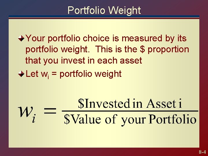
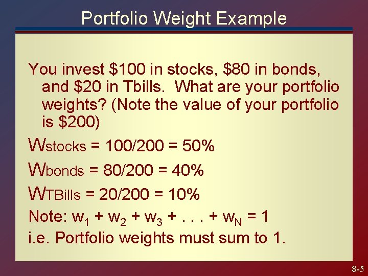
Portfolio Weight Your portfolio choice is measured by its portfolio weight. This is the $ proportion that you invest in each asset Let wi = portfolio weight 8 -4

Portfolio Weight Example You invest $100 in stocks, $80 in bonds, and $20 in Tbills. What are your portfolio weights? (Note the value of your portfolio is $200) Wstocks = 100/200 = 50% Wbonds = 80/200 = 40% WTBills = 20/200 = 10% Note: w 1 + w 2 + w 3 +. . . + w. N = 1 i. e. Portfolio weights must sum to 1. 8 -5

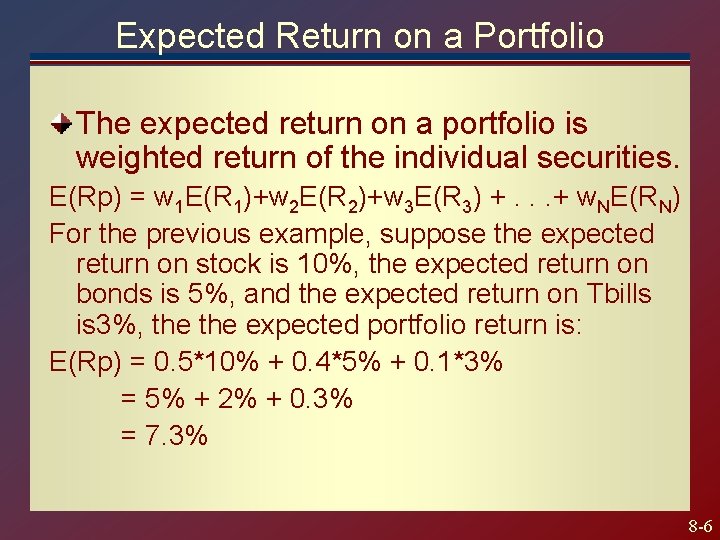
Expected Return on a Portfolio The expected return on a portfolio is weighted return of the individual securities. E(Rp) = w 1 E(R 1)+w 2 E(R 2)+w 3 E(R 3) +. . . + w. NE(RN) For the previous example, suppose the expected return on stock is 10%, the expected return on bonds is 5%, and the expected return on Tbills is 3%, the expected portfolio return is: E(Rp) = 0. 5*10% + 0. 4*5% + 0. 1*3% = 5% + 2% + 0. 3% = 7. 3% 8 -6

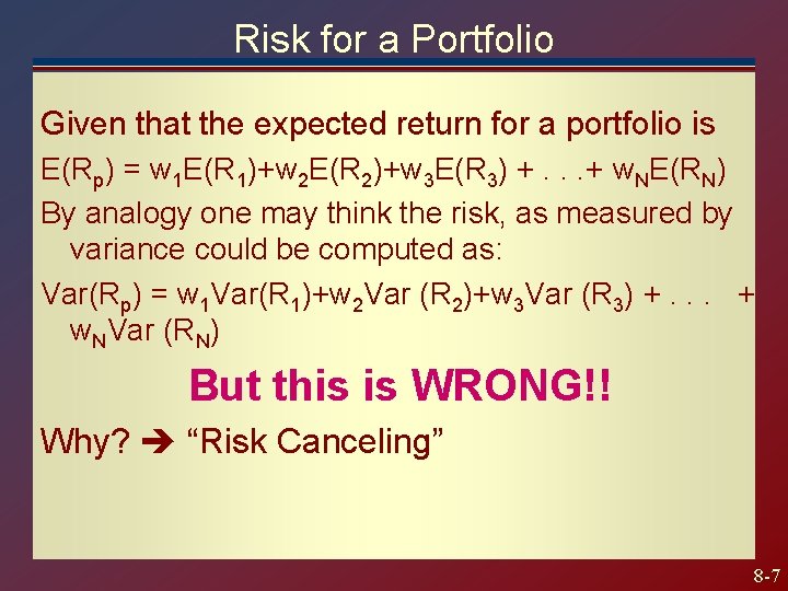
Risk for a Portfolio Given that the expected return for a portfolio is E(Rp) = w 1 E(R 1)+w 2 E(R 2)+w 3 E(R 3) +. . . + w. NE(RN) By analogy one may think the risk, as measured by variance could be computed as: Var(Rp) = w 1 Var(R 1)+w 2 Var (R 2)+w 3 Var (R 3) +. . . + w. NVar (RN) But this is WRONG!! Why? “Risk Canceling” 8 -7

A Contrived Example Asset YESPUR will pay $100 if the Spurs take the NBA championship next year, and zero otherwise Asset NOSPUR pays $100 if the Spurs do not win the NBA championship and pays zero otherwise. Both of the above assets are risky, as we do not know who will win the NBA this season 8 -8

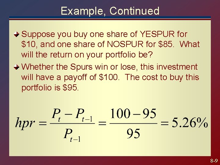
Example, Continued Suppose you buy one share of YESPUR for $10, and one share of NOSPUR for $85. What will the return on your portfolio be? Whether the Spurs win or lose, this investment will have a payoff of $100. The cost to buy this portfolio is $95. 8 -9

Example - Summary This example shows a case where one can combine two risky assets to create a risk free asset. In other words, it shows that judicious choice of risky assets can reduce overall portfolio risk In most cases, one cannot eliminate all risk in a portfolio, but one can reduce risk through judicious choices of which securities to include in your portfolio 8 -10

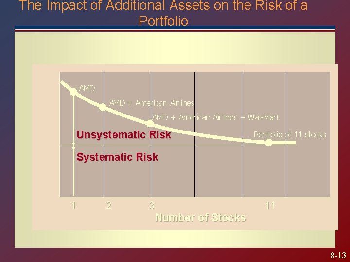
Diversification Most individual stock prices show higher volatility than the price volatility of portfolio of all common stocks. How can the standard deviation for individual stocks be higher than the standard deviation of the portfolio? Diversification: investing in many different assets reduces the volatility of the portfolio. The ups and downs of individual stocks partially cancel each other out. 8 -11

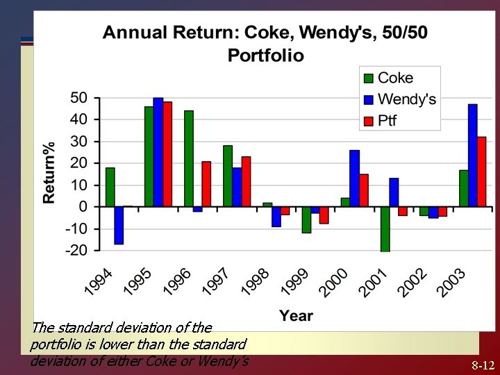
The standard deviation of the portfolio is lower than the standard deviation of either Coke or Wendy’s 8 -12

Portfolio Standard Deviation The Impact of Additional Assets on the Risk of a Portfolio AMD + American Airlines + Wal-Mart Unsystematic Risk Portfolio of 11 stocks Systematic Risk 1 2 3 11 Number of Stocks 8 -13

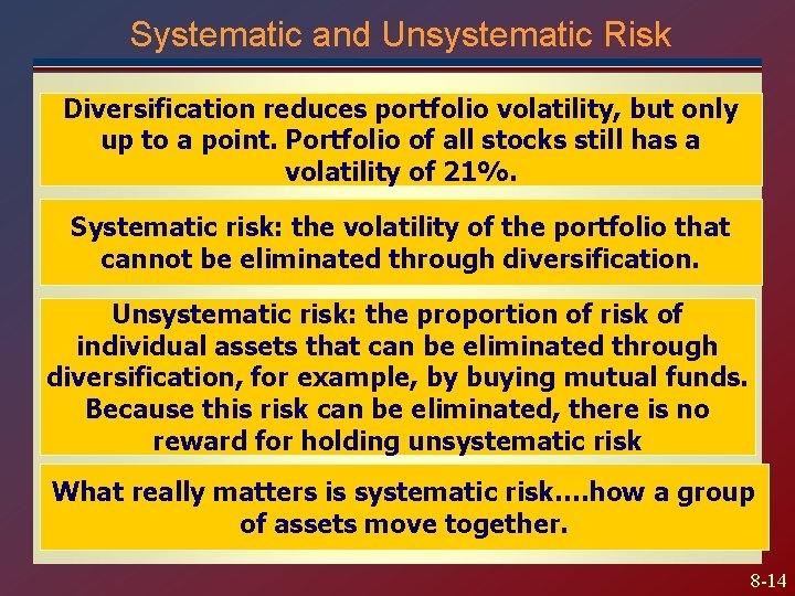
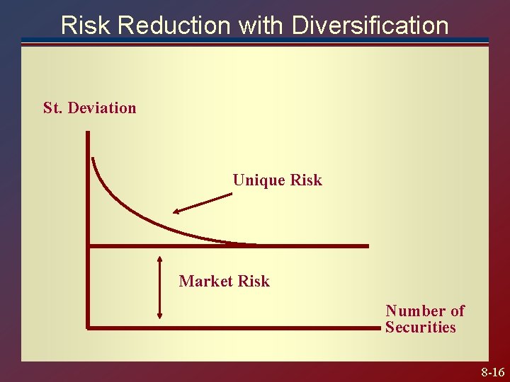
Systematic and Unsystematic Risk Diversification reduces portfolio volatility, but only up to a point. Portfolio of all stocks still has a volatility of 21%. Systematic risk: the volatility of the portfolio that cannot be eliminated through diversification. Unsystematic risk: the proportion of risk of individual assets that can be eliminated through diversification, for example, by buying mutual funds. Because this risk can be eliminated, there is no reward for holding unsystematic risk What really matters is systematic risk…. how a group of assets move together. 8 -14

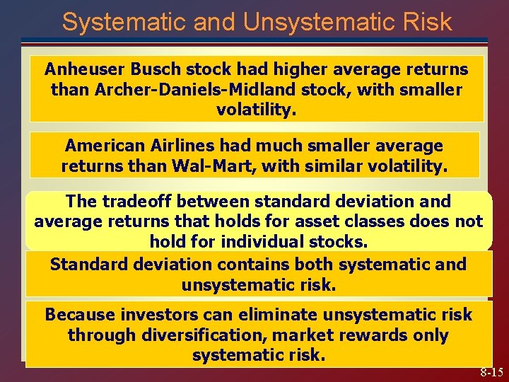
Systematic and Unsystematic Risk Anheuser Busch stock had higher average returns than Archer-Daniels-Midland stock, with smaller volatility. American Airlines had much smaller average returns than Wal-Mart, with similar volatility. The tradeoff between standard deviation and average returns that holds for asset classes does not hold for individual stocks. Standard deviation contains both systematic and unsystematic risk. Because investors can eliminate unsystematic risk through diversification, market rewards only systematic risk. 8 -15

Risk Reduction with Diversification St. Deviation Unique Risk Market Risk Number of Securities 8 -16

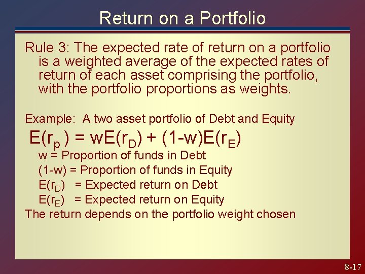
Return on a Portfolio Rule 3: The expected rate of return on a portfolio is a weighted average of the expected rates of return of each asset comprising the portfolio, with the portfolio proportions as weights. Example: A two asset portfolio of Debt and Equity E(rp ) = w. E(r. D) + (1 -w)E(r. E) w = Proportion of funds in Debt (1 -w) = Proportion of funds in Equity E(r. D) = Expected return on Debt E(r. E) = Expected return on Equity The return depends on the portfolio weight chosen 8 -17

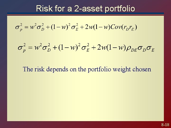
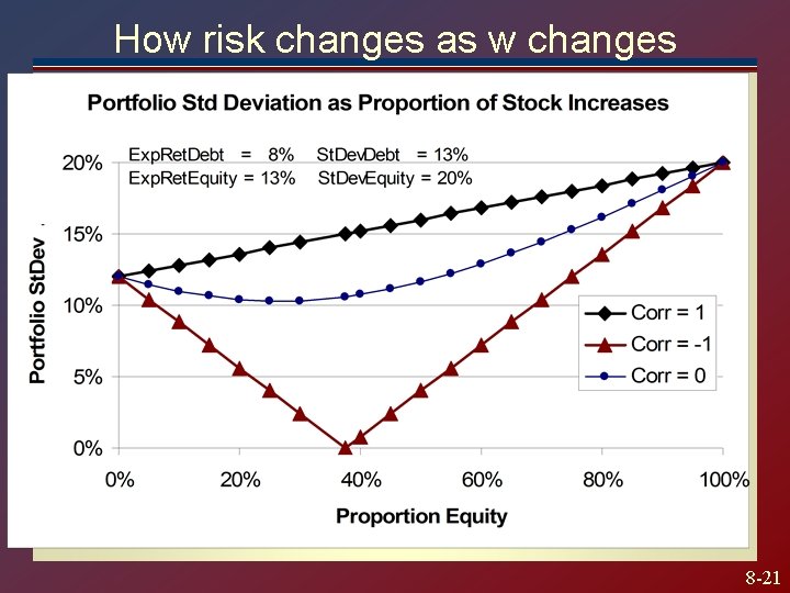
Risk for a 2 -asset portfolio The risk depends on the portfolio weight chosen 8 -18

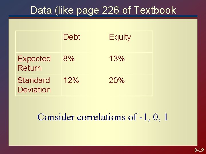
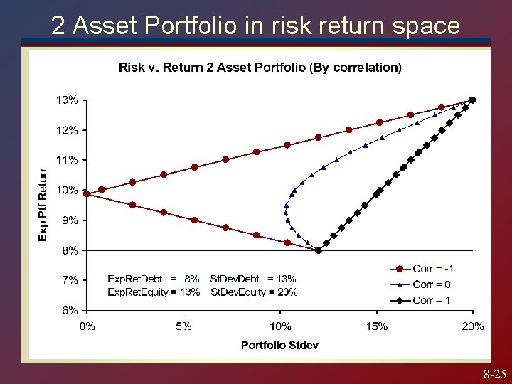
Data (like page 226 of Textbook Debt Equity Expected Return 8% 13% Standard Deviation 12% 20% Consider correlations of -1, 0, 1 8 -19

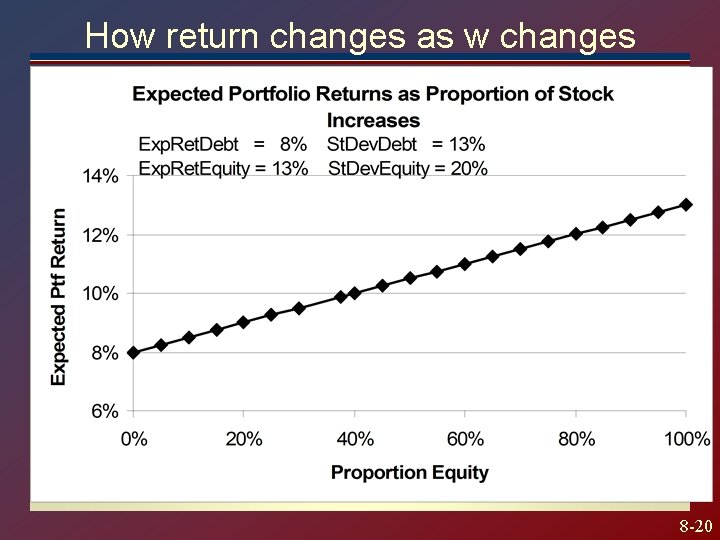
How return changes as w changes 8 -20

How risk changes as w changes 8 -21

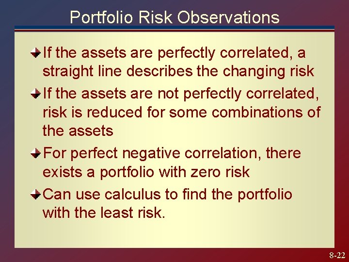
Portfolio Risk Observations If the assets are perfectly correlated, a straight line describes the changing risk If the assets are not perfectly correlated, risk is reduced for some combinations of the assets For perfect negative correlation, there exists a portfolio with zero risk Can use calculus to find the portfolio with the least risk. 8 -22

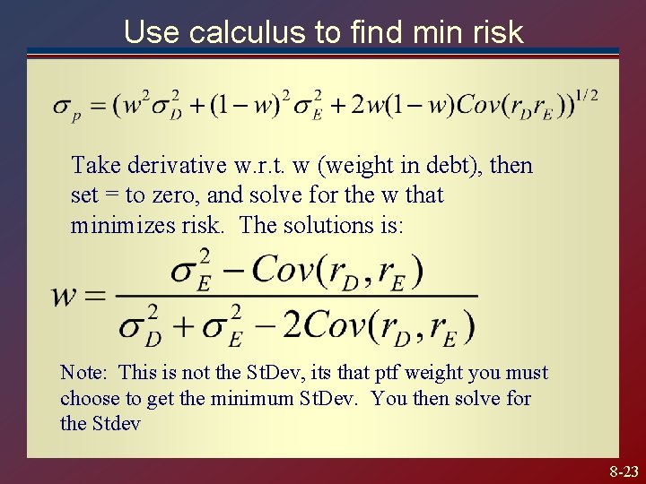
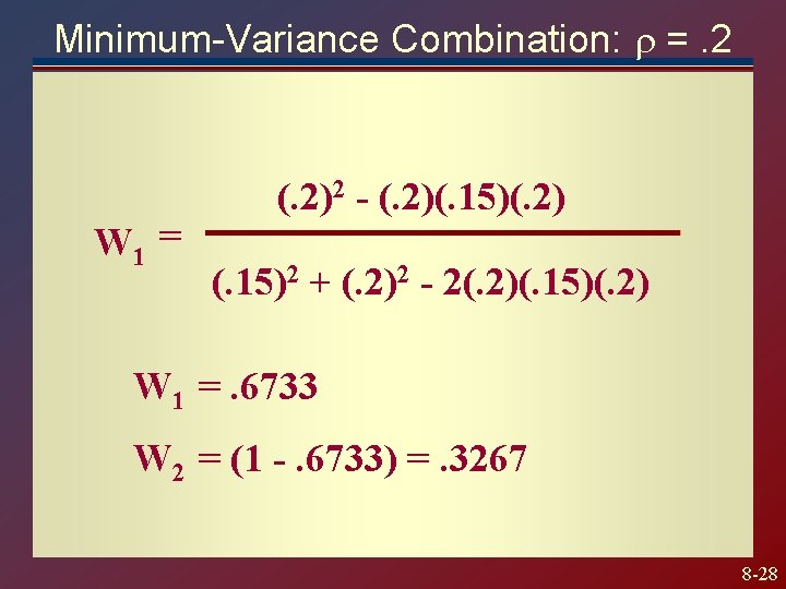
Use calculus to find min risk Take derivative w. r. t. w (weight in debt), then set = to zero, and solve for the w that minimizes risk. The solutions is: Note: This is not the St. Dev, its that ptf weight you must choose to get the minimum St. Dev. You then solve for the Stdev 8 -23

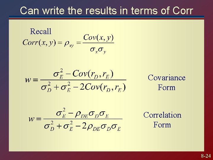
Can write the results in terms of Corr Recall Covariance Form Correlation Form 8 -24

2 Asset Portfolio in risk return space 8 -25

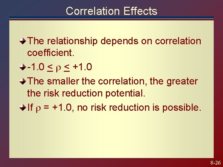
Correlation Effects The relationship depends on correlation coefficient. -1. 0 < < +1. 0 The smaller the correlation, the greater the risk reduction potential. If = +1. 0, no risk reduction is possible. 8 -26

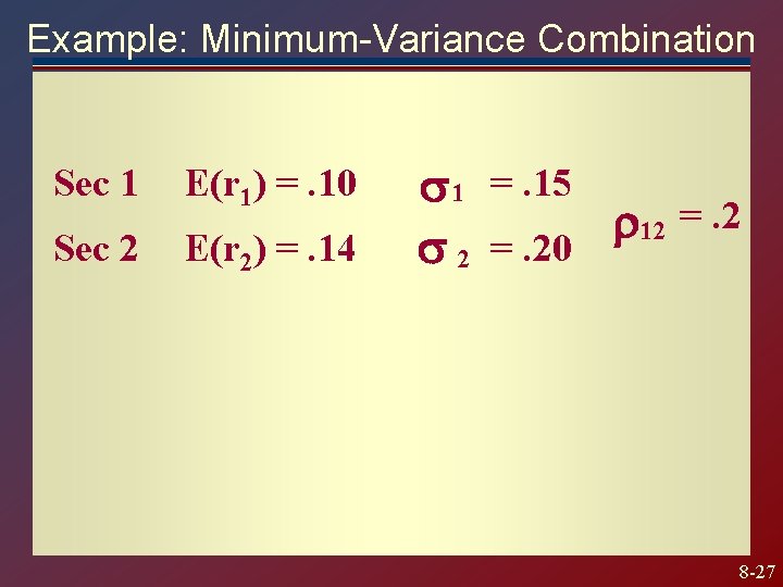
Example: Minimum-Variance Combination Sec 1 E(r 1) =. 10 Sec 2 E(r 2) =. 14 1 =. 15 12 =. 2 2 =. 20 8 -27

Minimum-Variance Combination: =. 2 W 1 = (. 2)2 - (. 2)(. 15)(. 2) (. 15)2 + (. 2)2 - 2(. 2)(. 15)(. 2) W 1 =. 6733 W 2 = (1 -. 6733) =. 3267 8 -28

Risk and Return: Minimum Variance rp =. 6733(. 10) +. 3267(. 14) =. 1131 p = [(. 6733)2(. 15)2 + (. 3267)2(. 2)2 + 2(. 6733)(. 3267)(. 2)(. 15)(. 2)] p = [. 0171] 1/2 =. 1308 8 -29

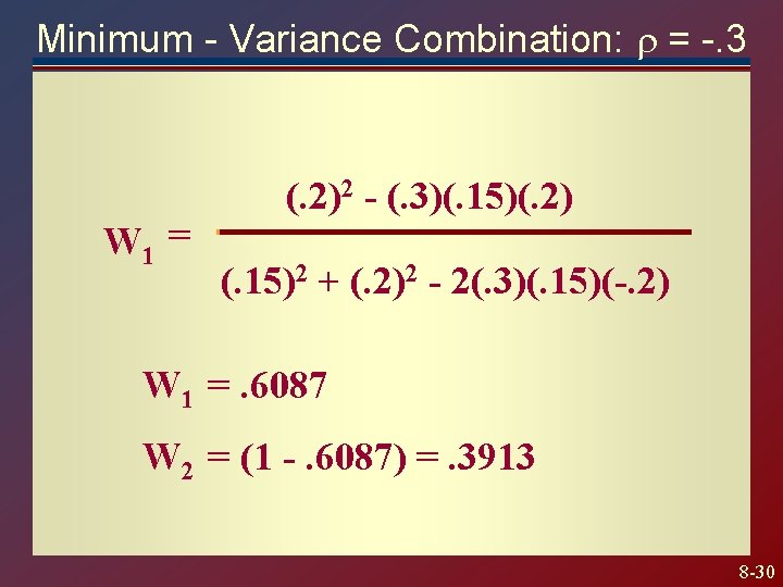
Minimum - Variance Combination: = -. 3 W 1 = (. 2)2 - (. 3)(. 15)(. 2) (. 15)2 + (. 2)2 - 2(. 3)(. 15)(-. 2) W 1 =. 6087 W 2 = (1 -. 6087) =. 3913 8 -30

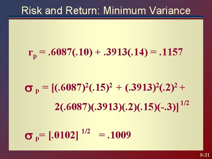
Risk and Return: Minimum Variance rp =. 6087(. 10) +. 3913(. 14) =. 1157 p = [(. 6087)2(. 15)2 + (. 3913)2(. 2)2 + 2(. 6087)(. 3913)(. 2)(. 15)(-. 3)] p= [. 0102] 1/2 =. 1009 8 -31

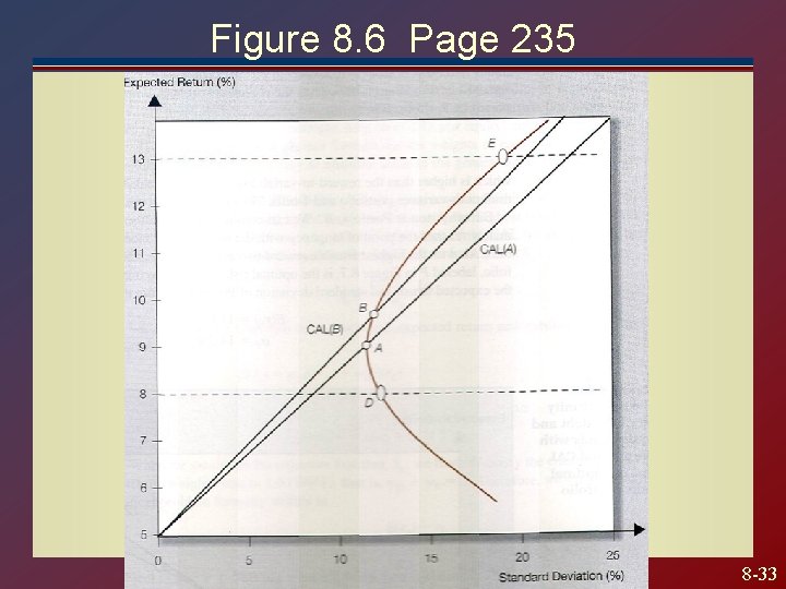
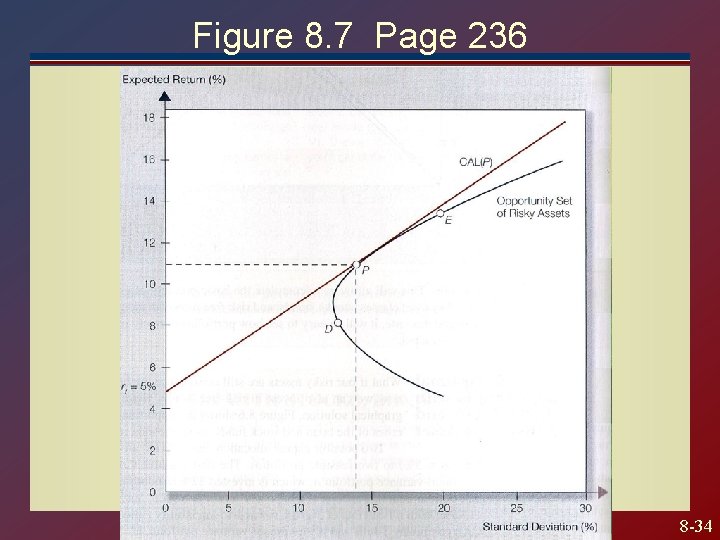
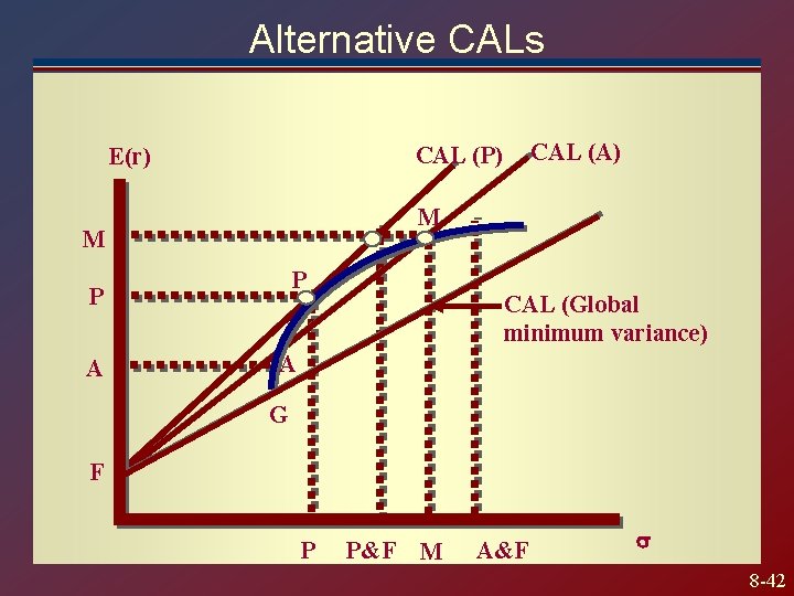
Adding a Risk Free Asset With the addition of the risk free asset, to create a complete portfolio, we can create an infinite number of CAL’s by drawing a straight line from the Rf to the portfolio. To prevent mean variance dominance, however, only the CAL with the maximum slope will be non dominated Finding the efficient CAL is a calculus problem 8 -32

Figure 8. 6 Page 235 8 -33

Figure 8. 7 Page 236 8 -34

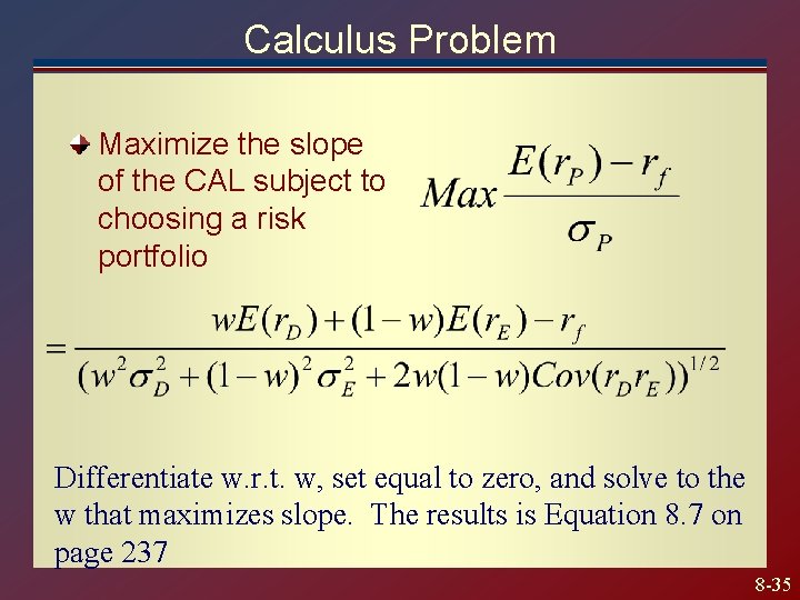
Calculus Problem Maximize the slope of the CAL subject to choosing a risk portfolio Differentiate w. r. t. w, set equal to zero, and solve to the w that maximizes slope. The results is Equation 8. 7 on page 237 8 -35

Solve for optimal risky portfolio Using Equation 8. 7 you can solve for the optimal risky portfolio, in terms of E(r) and Standard Deviation. You can then use this information to compute the slope of the CAL. Complete portfolios will be combination of this optimal portfolio and the risk free asset 8 -36

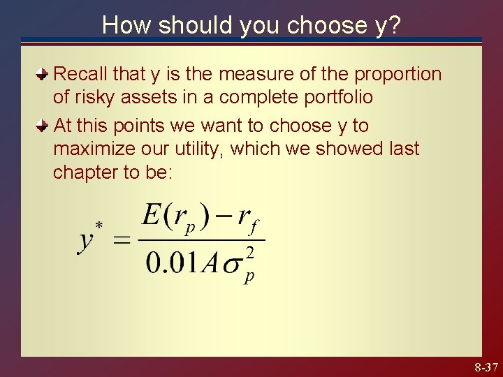
How should you choose y? Recall that y is the measure of the proportion of risky assets in a complete portfolio At this points we want to choose y to maximize our utility, which we showed last chapter to be: 8 -37

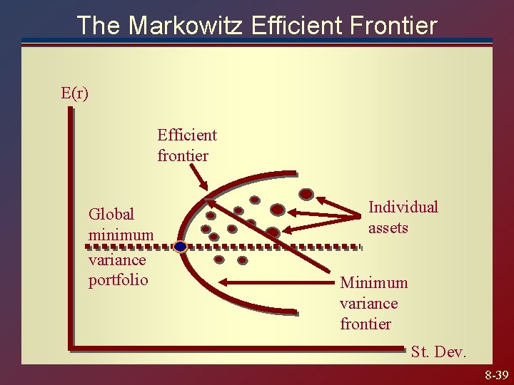
Extending Concepts to All Securities First plot all risky assets Then draw the two asset portfolios for each of the combination (depend on Corr) The outer locus of points will have the highest return for any level of risk, and are thus mean variance dominate These optimal portfolios are called the Markowitz efficient frontier. These portfolios are mean variance dominant. 8 -38

The Markowitz Efficient Frontier E(r) Efficient frontier Global minimum variance portfolio Individual assets Minimum variance frontier St. Dev. 8 -39

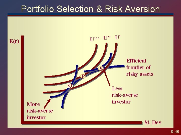
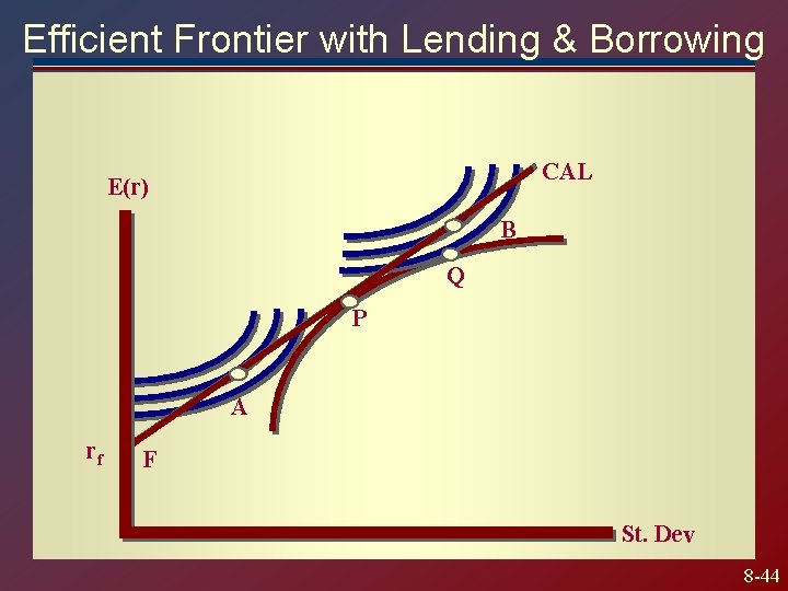
Portfolio Selection & Risk Aversion U’’’ U’ E(r) S P Q More risk-averse investor Efficient frontier of risky assets Less risk-averse investor St. Dev 8 -40

Extending to Include Riskless Asset The set up is the same as when there was simply 2 risky assets. In other words there is a point that will maximize the slope of a CAL, and this represents the optimal mix of risky securities to hold along with the risk free asset 8 -41

Alternative CALs M M P P A CAL (A) CAL (P) E(r) CAL (Global minimum variance) A G F P P&F M A&F 8 -42

The separation property Because one CAL dominates the frontier of risky asset portfolios, all investors will choose to invest in the same risk portfolio and then will choose varying amounts of the risk free asset to maximize utility. Portfolio analysis can be separeted into two tasks 1. Determine the optimal risk portfolio (This mutual fund can serve all investors) 2. Choose the asset allocation of the risk free versus the risky portfolio 8 -43

Efficient Frontier with Lending & Borrowing CAL E(r) B Q P A rf F St. Dev 8 -44

Differential Borrowing and Lending Rates 8 -45