Optimal Multilevel System Design under Uncertainty M Kokkolaras

Optimal Multilevel System Design under Uncertainty M. Kokkolaras and P. Y Papalambros University of Michigan Z. Mourelatos Oakland University NSF Workshop on Reliable Engineering Computing Savannah, Georgia, 16 September 2004

Outline • Design by Decomposition • Hierarchical Multilevel Systems • Analytical Target Cascading – Deterministic Formulation – Nondeterministic Formulations • Propagation of Uncertainty • Practical Issues • Example

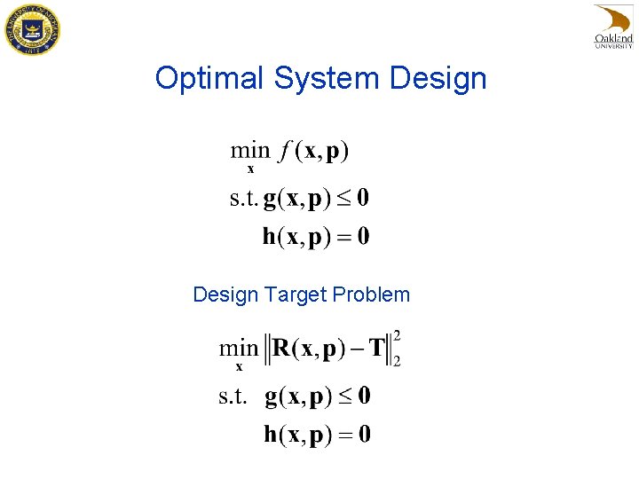
Optimal System Design Target Problem

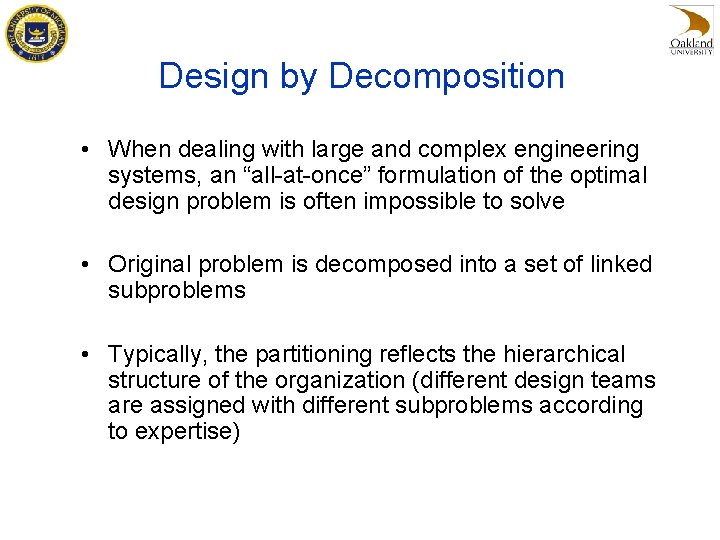
Design by Decomposition • When dealing with large and complex engineering systems, an “all-at-once” formulation of the optimal design problem is often impossible to solve • Original problem is decomposed into a set of linked subproblems • Typically, the partitioning reflects the hierarchical structure of the organization (different design teams are assigned with different subproblems according to expertise)

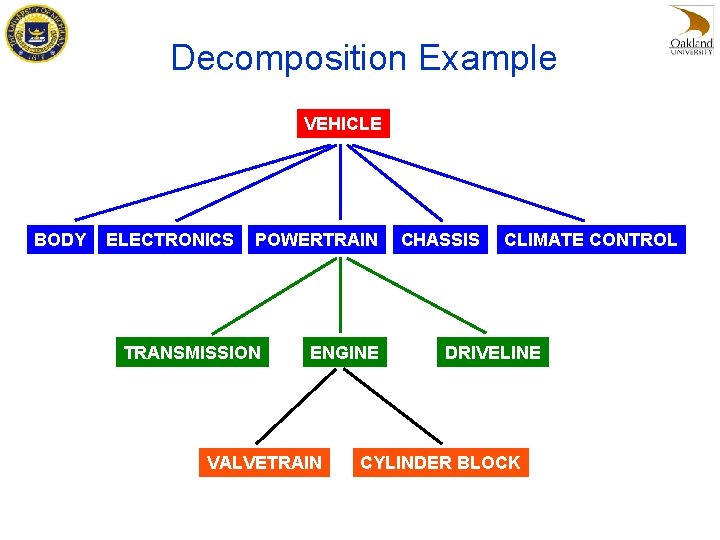
Decomposition Example VEHICLE BODY ELECTRONICS POWERTRAIN TRANSMISSION ENGINE … VALVETRAIN CHASSIS CLIMATE CONTROL DRIVELINE CYLINDER BLOCK

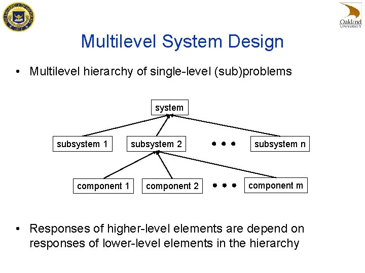
Multilevel System Design • Multilevel hierarchy of single-level (sub)problems system subsystem 1 component 1 subsystem 2 component 2 subsystem n component m • Responses of higher-level elements are depend on responses of lower-level elements in the hierarchy

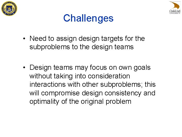
Challenges • Need to assign design targets for the subproblems to the design teams • Design teams may focus on own goals without taking into consideration interactions with other subproblems; this will compromise design consistency and optimality of the original problem

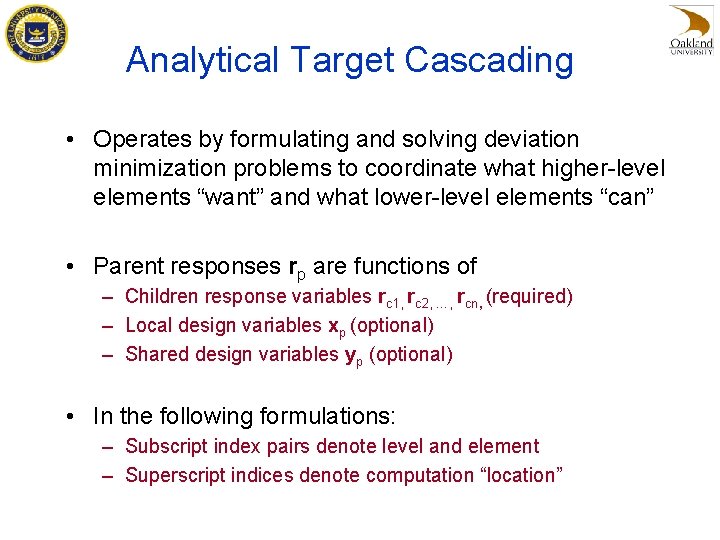
Analytical Target Cascading • Operates by formulating and solving deviation minimization problems to coordinate what higher-level elements “want” and what lower-level elements “can” • Parent responses rp are functions of – Children response variables rc 1, rc 2, …, rcn, (required) – Local design variables xp (optional) – Shared design variables yp (optional) • In the following formulations: – Subscript index pairs denote level and element – Superscript indices denote computation “location”

Mathematical Formulation

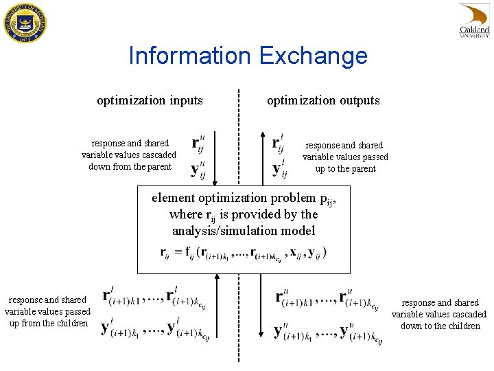
Information Exchange optimization inputs response and shared variable values cascaded down from the parent optimization outputs response and shared variable values passed up to the parent element optimization problem pij, where rij is provided by the analysis/simulation model response and shared variable values passed up from the children response and shared variable values cascaded down to the children

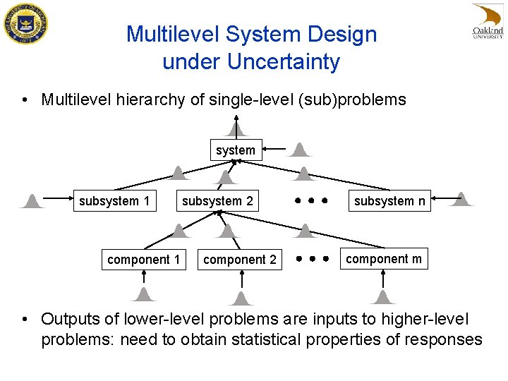
Multilevel System Design under Uncertainty • Multilevel hierarchy of single-level (sub)problems system subsystem 1 component 1 subsystem 2 component 2 subsystem n component m • Outputs of lower-level problems are inputs to higher-level problems: need to obtain statistical properties of responses

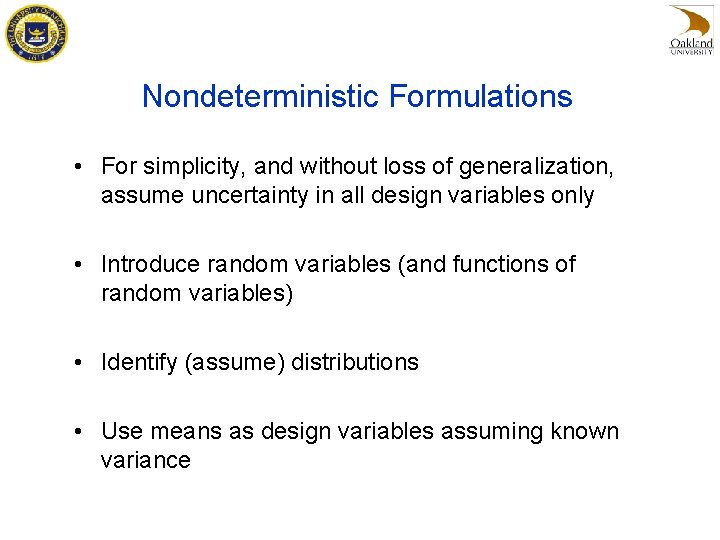
Nondeterministic Formulations • For simplicity, and without loss of generalization, assume uncertainty in all design variables only • Introduce random variables (and functions of random variables) • Identify (assume) distributions • Use means as design variables assuming known variance

Stochastic Formulation

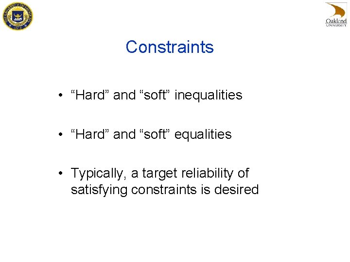
Constraints • “Hard” and “soft” inequalities • “Hard” and “soft” equalities • Typically, a target reliability of satisfying constraints is desired

Probabilistic Formulation

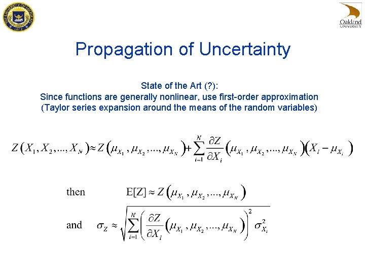
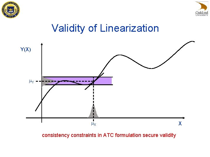
Propagation of Uncertainty State of the Art (? ): Since functions are generally nonlinear, use first-order approximation (Taylor series expansion around the means of the random variables)

Validity of Linearization Y(X) m. Y m. X consistency constraints in ATC formulation secure validity X

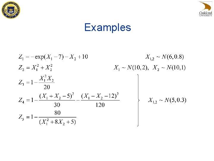
Examples

Results E[Z 1] Var[Z 1]1/2 E[Z 2] Var[Z 2]1/2 E[Z 3] Var[Z 3]1/2 E[Z 4] Var[Z 4]1/2 E[Z 5] Var[Z 5]1/2 * 1, 000 samples Linear. MCS* elin % 3. 6321 1. 9386 200 44. 721 -5. 25 0. 8385 -1. 0333 0. 1166 -0. 1428 0. 00627 3. 4921 0. 9327 205. 04 45. 101 -5. 3114 0. 8407 -1. 0404 0. 1653 -0. 1448 0. 00630 4. 00 107. 85 -2. 45 -0. 84 -1. 15 -0. 26 -0. 68 29. 46 -1. 3 -0. 47

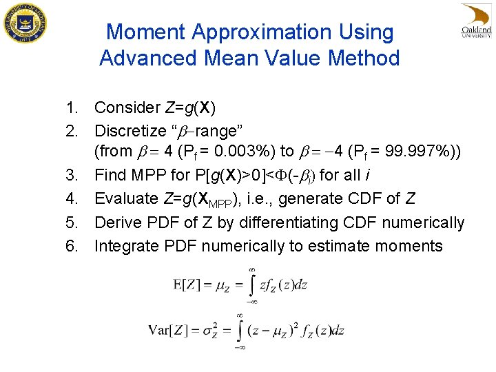
Moment Approximation Using Advanced Mean Value Method 1. Consider Z=g(X) 2. Discretize “b-range” (from b = 4 (Pf = 0. 003%) to b = -4 (Pf = 99. 997%)) 3. Find MPP for P[g(X)>0]<F(-bi) for all i 4. Evaluate Z=g(XMPP), i. e. , generate CDF of Z 5. Derive PDF of Z by differentiating CDF numerically 6. Integrate PDF numerically to estimate moments

Results Linear. E[Z 1] Var[Z 1]1/2 E[Z 2] Var[Z 2]1/2 E[Z 3] Var[Z 3]1/2 E[Z 4] Var[Z 4]1/2 E[Z 5] Var[Z 5]1/2 * 3. 6321 1. 9386 200 44. 721 -5. 25 0. 8385 -1. 0333 0. 1166 -0. 1428 0. 00627 1, 000 samples MAM MCS* 3. 6029 3. 4921 0. 9013 0. 9327 203. 37 205. 04 45. 203 45. 101 -5. 3495 -5. 3114 0. 8423 0. 8407 -1. 0380 -1. 0404 0. 1653 -0. 1454 -0. 1448 0. 00631 0. 00630 elin % e. MAM % 4. 00 107. 85 -2. 45 -0. 84 -1. 15 -0. 26 -0. 68 29. 46 -1. 3 -0. 47 3. 17 -3. 36 -0. 81 0. 22 0. 71 0. 19 -0. 23 0 0. 41 0. 15

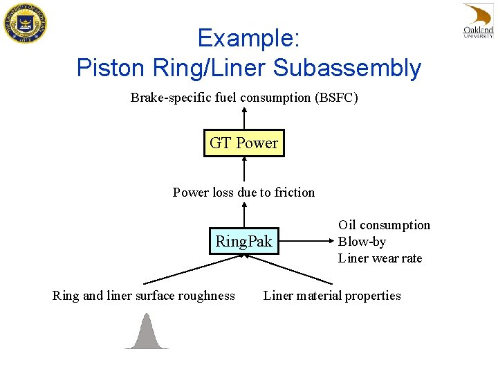
Example: Piston Ring/Liner Subassembly Brake-specific fuel consumption (BSFC) GT Power loss due to friction Ring. Pak Ring and liner surface roughness Oil consumption Blow-by Liner wear rate Liner material properties

Lower-level Problem Formulation

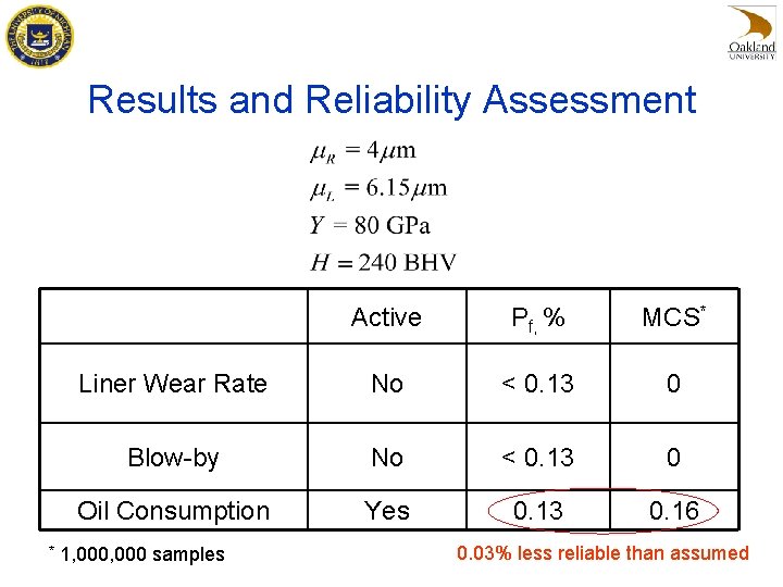
Results and Reliability Assessment * Active Pf, % MCS* Liner Wear Rate No < 0. 13 0 Blow-by No < 0. 13 0 Oil Consumption Yes 0. 13 0. 16 1, 000 samples 0. 03% less reliable than assumed

Statistical Properties of Power Loss E[pl] Var[pl]1/2 Linearization MAM 0. 3950 0. 3922 0. 0481 0. 0309 MAM - PDF MCS 0. 3932 0. 0311 Lin. e 0. 45% 54. 6% MAM e -0. 25% -0. 64% MCS – PDF (1, 000 samples)

Upper-level Problem Formulation * Lin. e MAM e Linearization MAM MCS* E[fuel] 0. 5341 0. 5342 Var[fuel]1/2 0. 00757 0. 00760 0. 00759 -0. 25% 0. 13% 1, 000 samples -0. 01%

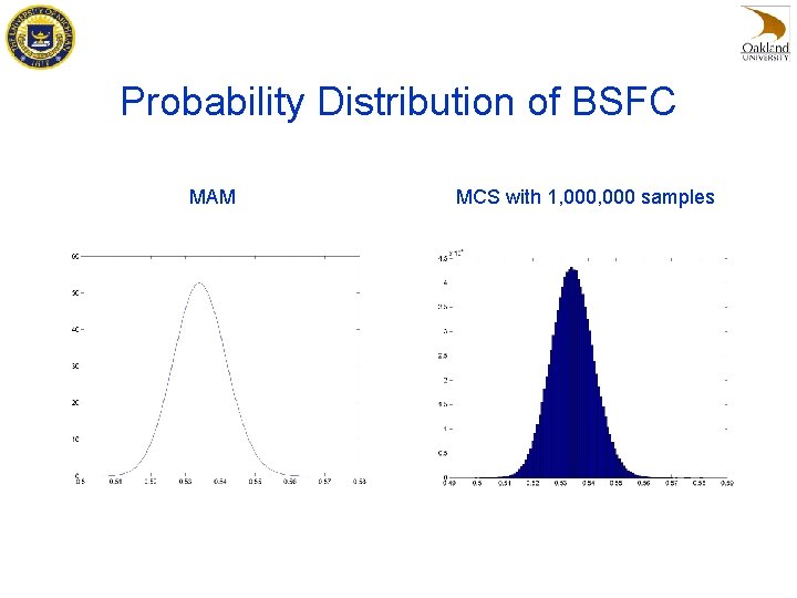
Probability Distribution of BSFC MAM MCS with 1, 000 samples

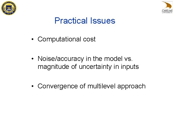
Practical Issues • Computational cost • Noise/accuracy in the model vs. magnitude of uncertainty in inputs • Convergence of multilevel approach

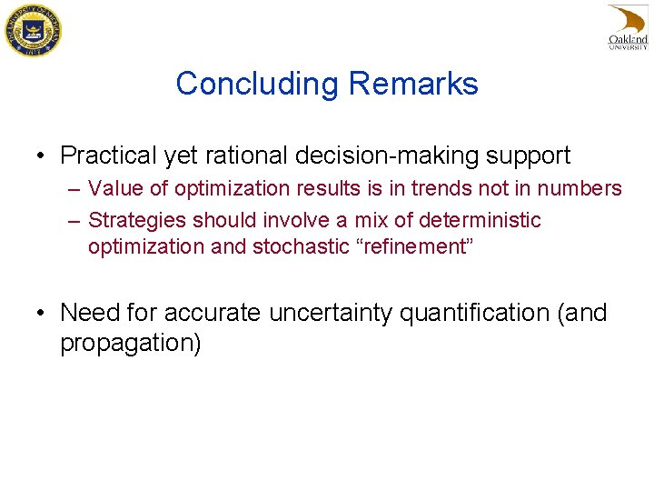
Concluding Remarks • Practical yet rational decision-making support – Value of optimization results is in trends not in numbers – Strategies should involve a mix of deterministic optimization and stochastic “refinement” • Need for accurate uncertainty quantification (and propagation)

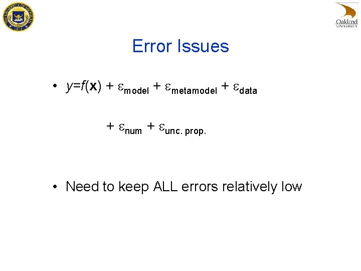
Error Issues • y=f(x) + emodel + emetamodel + edata + enum + eunc. prop. • Need to keep ALL errors relatively low

Q&A

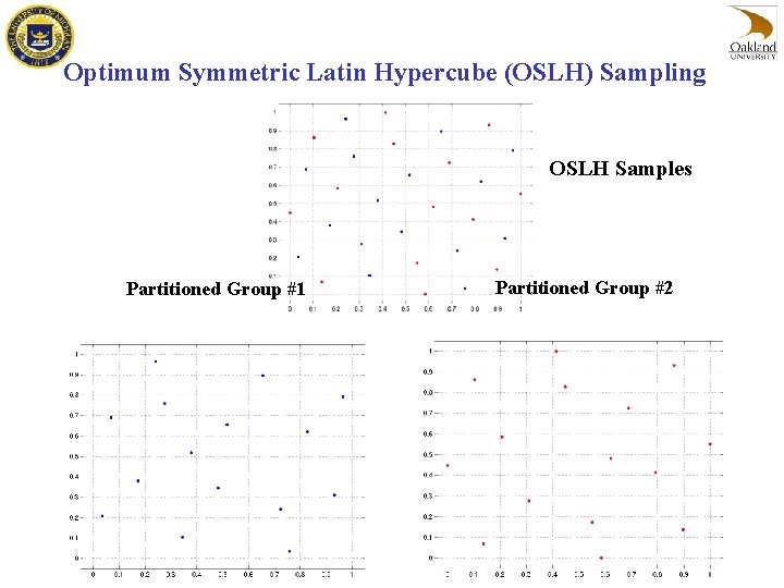
Optimum Symmetric Latin Hypercube (OSLH) Sampling OSLH Samples Partitioned Group #1 Partitioned Group #2

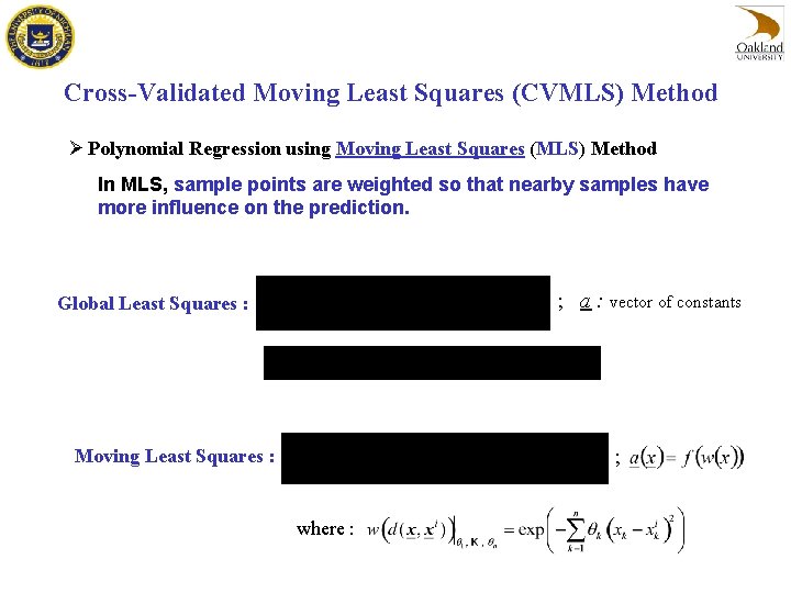
Cross-Validated Moving Least Squares (CVMLS) Method Ø Polynomial Regression using Moving Least Squares (MLS) Method In MLS, sample points are weighted so that nearby samples have more influence on the prediction. ; a : vector of constants Global Least Squares : ; Moving Least Squares : where :

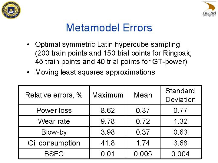
Metamodel Errors • Optimal symmetric Latin hypercube sampling (200 train points and 150 trial points for Ringpak, 45 train points and 40 trial points for GT-power) • Moving least squares approximations Relative errors, % Maximum Mean Standard Deviation Power loss Wear rate Blow-by Oil consumption BSFC 8. 62 9. 78 3. 98 41. 8 0. 01 0. 37 0. 72 0. 37 1. 74 0. 005 0. 77 1. 32 0. 63 3. 68 0. 004

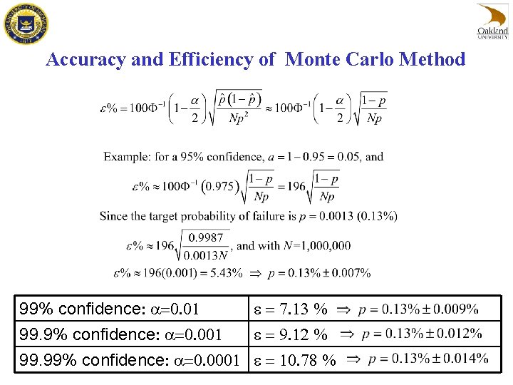
Accuracy and Efficiency of Monte Carlo Method 99% confidence: a=0. 01 e = 7. 13 % 99. 9% confidence: a=0. 001 e = 9. 12 % 99. 99% confidence: a=0. 0001 e = 10. 78 %