Optimal Income Taxation When Top Income Inequality Increases

Optimal Income Taxation When Top Income Inequality Increases Matti Tuomala 22. 9. 2016 SIEP, LECCE

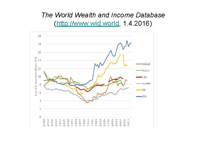
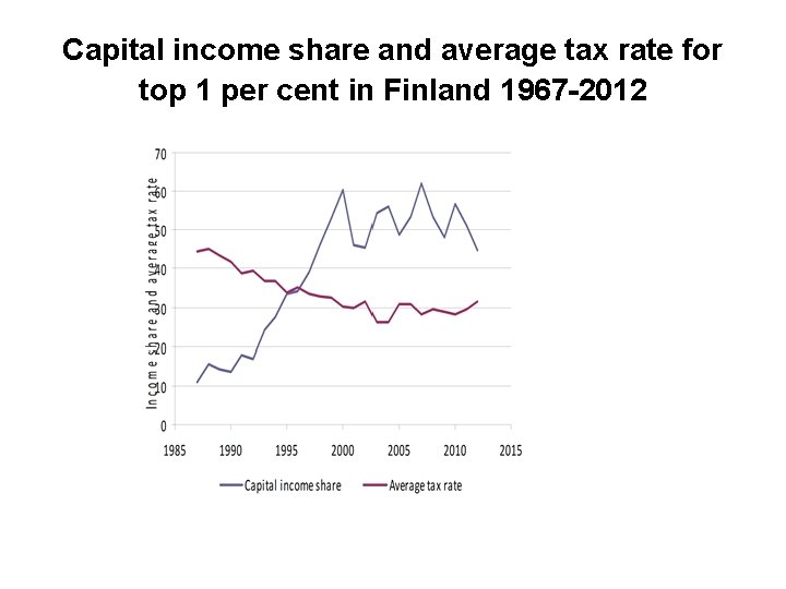
Taxes and Top income inequality • At the same time with a large growth in top income shares over the past few decades there has been in many advanced countries a shift in the burden of taxation from the top to the further down in the income distribution. • Piketty et al. (2011, 2014) find in OECD countries a strong correlation between tax cuts for the highest earners and increases in the income share of the top 1 per cent since 1975.

The World Wealth and Income Database (http: //www. wid. world, 1. 4. 2016)

Top tax rates 1967– 2010). Data source: Piketty, Saez and Stantcheva (2011; 2014).

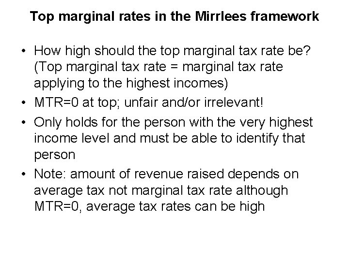
Top marginal rates in the Mirrlees framework • How high should the top marginal tax rate be? (Top marginal tax rate = marginal tax rate applying to the highest incomes) • MTR=0 at top; unfair and/or irrelevant! • Only holds for the person with the very highest income level and must be able to identify that person • Note: amount of revenue raised depends on average tax not marginal tax rate although MTR=0, average tax rates can be high

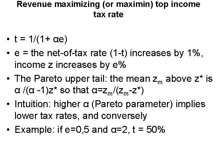
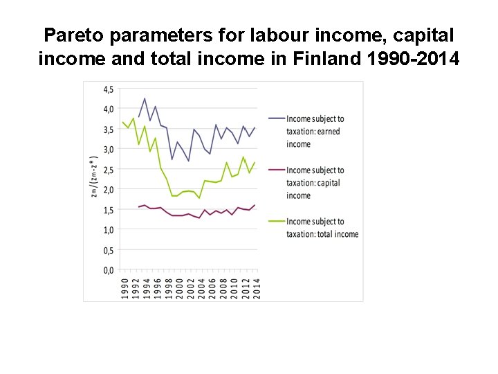
Revenue maximizing (or maximin) top income tax rate • t = 1/(1+ αe) • e = the net-of-tax rate (1 -t) increases by 1%, income z increases by e% • The Pareto upper tail: the mean zm above z* is α /(α -1)z* so that α=zm/(zm-z*) • Intuition: higher α (Pareto parameter) implies lower tax rates, and conversely • Example: if e=0, 5 and α=2, t = 50%

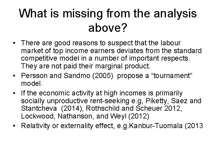
What is missing from the analysis above? • There are good reasons to suspect that the labour market of top income earners deviates from the standard competitive model in a number of important respects. They are not paid their marginal product. • Persson and Sandmo (2005) propose a “tournament” model. • If the economic activity at high incomes is primarily socially unproductive rent-seeking e. g, Piketty, Saez and Stantcheva (2014), Rothschild and Scheuer 2012, Lockwood, Nathanson, and Weyl (2012) • Relativity or externality effect, e. g. Kanbur-Tuomala (2013

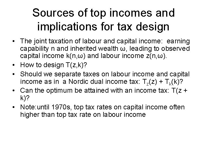
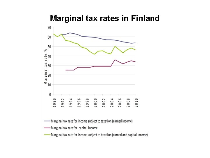
Sources of top incomes and implications for tax design • The joint taxation of labour and capital income: earning capability n and inherited wealth ω, leading to observed capital income k(n, ω) and labour income z(n, ω). • How to design T(z, k)? • Should we separate taxes on labour income and capital income as in a Nordic dual income tax: Tz(z) + Tk(k)? • Can the optimum be attained with an income tax: T(z + k)? • Note: until 1970 s, top tax rates on capital income often higher than top tax rate on labour income

Marginal tax rates in Finland

Capital income share and average tax rate for top 1 per cent in Finland 1967 -2012

Pareto parameters for labour income, capital income and total income in Finland 1990 -2014

Separable schedules in labour and capital income: T(z) + T(k) Maximin case • As in Christiansen-Tuomala (2008) we consider a two-period model wherein an individual starts out with the endowment ω. • Individuals are free to divide their first period (when young) endowment between consumption, and savings. • Each unit of savings yields a consumer additional units of consumption in the second period.

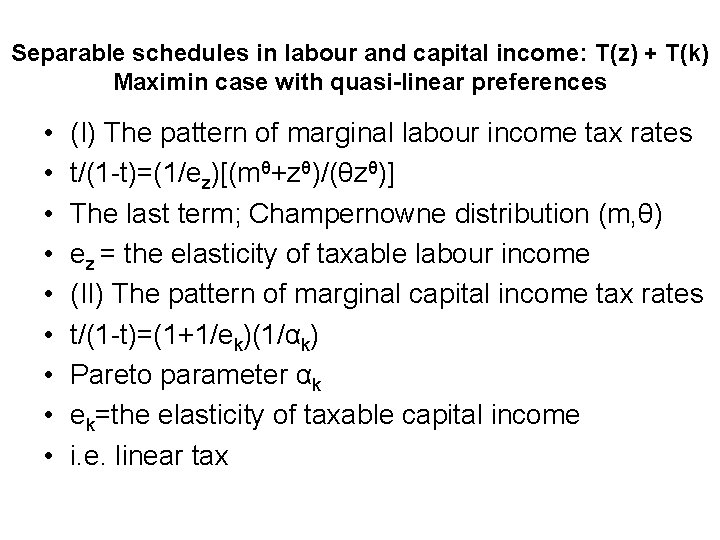
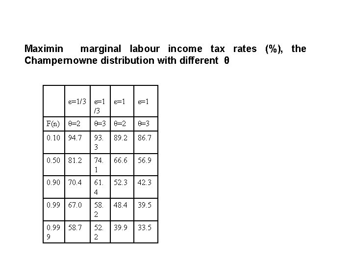
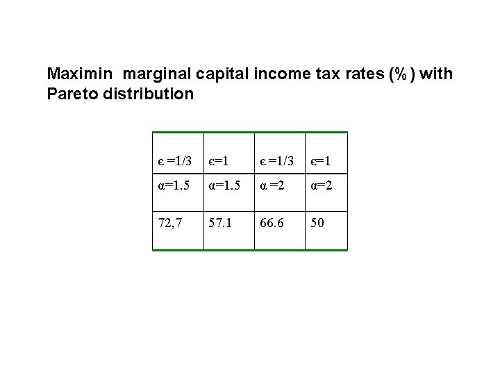
Separable schedules in labour and capital income: T(z) + T(k) Maximin case with quasi-linear preferences • • • (I) The pattern of marginal labour income tax rates t/(1 -t)=(1/ez)[(mθ+zθ)/(θzθ)] The last term; Champernowne distribution (m, θ) ez = the elasticity of taxable labour income (II) The pattern of marginal capital income tax rates t/(1 -t)=(1+1/ek)(1/αk) Pareto parameter αk ek=the elasticity of taxable capital income i. e. linear tax

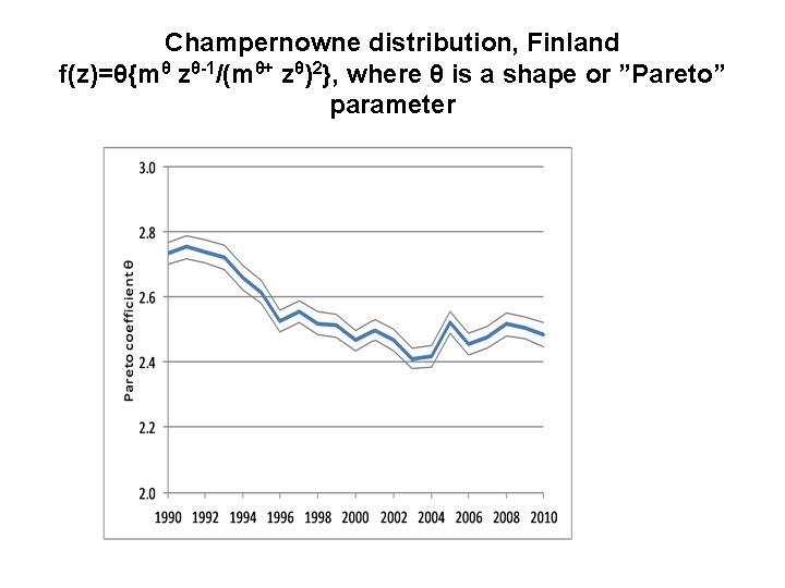
Champernowne distribution, Finland f(z)=θ{mθ zθ-1/(mθ+ zθ)2}, where θ is a shape or ”Pareto” parameter

Maximin marginal labour income tax rates (%), the Champernowne distribution with different θ є=1/3 є=1 є=1 F(n) θ=2 θ=3 0. 10 94. 7 93. 3 89. 2 86. 7 0. 50 81. 2 74. 1 66. 6 56. 9 0. 90 70. 4 61. 4 52. 3 42. 3 0. 99 67. 0 58. 2 48. 4 39. 5 0. 99 9 58. 7 52. 2 39. 9 33. 5

Maximin marginal capital income tax rates (%) with Pareto distribution є =1/3 є=1 α=1. 5 α =2 α=2 72, 7 57. 1 66. 6 50

Top income inequality and average tax rates • The top marginal rates are in itself important. • The more relevant tax rates for redistributive purposes are average tax rates. • The computational techniques can be used to say something about average rates.

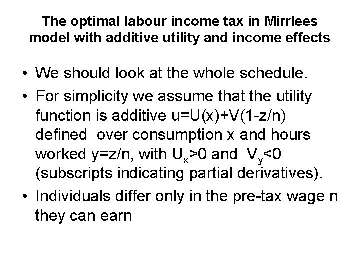
The optimal labour income tax in Mirrlees model with additive utility and income effects • We should look at the whole schedule. • For simplicity we assume that the utility function is additive u=U(x)+V(1 -z/n) defined over consumption x and hours worked y=z/n, with Ux>0 and Vy<0 (subscripts indicating partial derivatives). • Individuals differ only in the pre-tax wage n they can earn

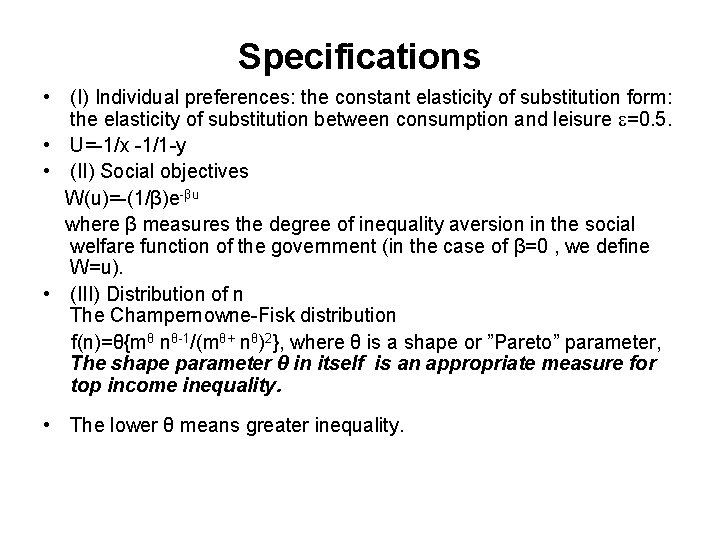
Specifications • (I) Individual preferences: the constant elasticity of substitution form: the elasticity of substitution between consumption and leisure =0. 5. • U=-1/x -1/1 -y • (II) Social objectives W(u)=-(1/β)e-βu where β measures the degree of inequality aversion in the social welfare function of the government (in the case of β=0 , we define W=u). • (III) Distribution of n The Champernowne-Fisk distribution f(n)=θ{mθ nθ-1/(mθ+ nθ)2}, where θ is a shape or ”Pareto” parameter, The shape parameter θ in itself is an appropriate measure for top income inequality. • The lower θ means greater inequality.

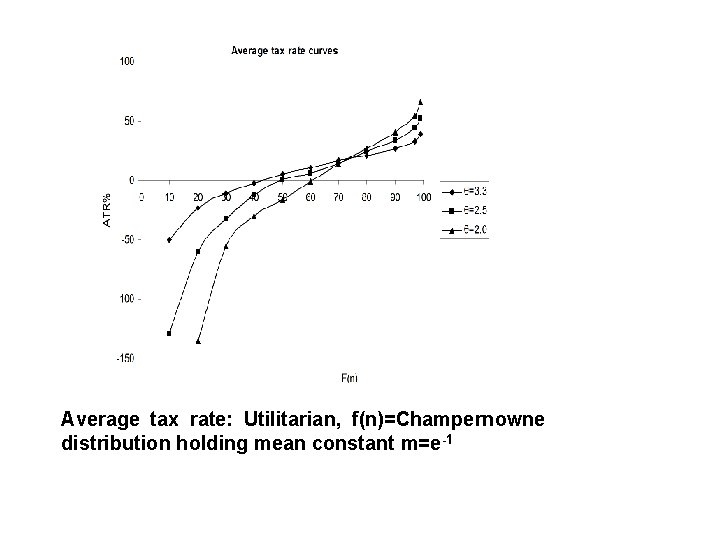
Average tax rate: Utilitarian, f(n)=Champernowne distribution holding mean constant m=e-1

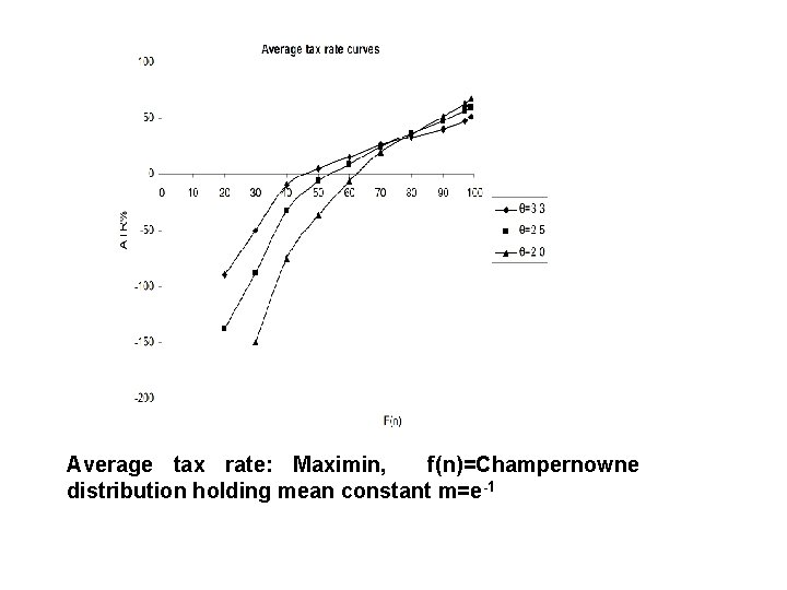
Average tax rate: Maximin, f(n)=Champernowne distribution holding mean constant m=e-1

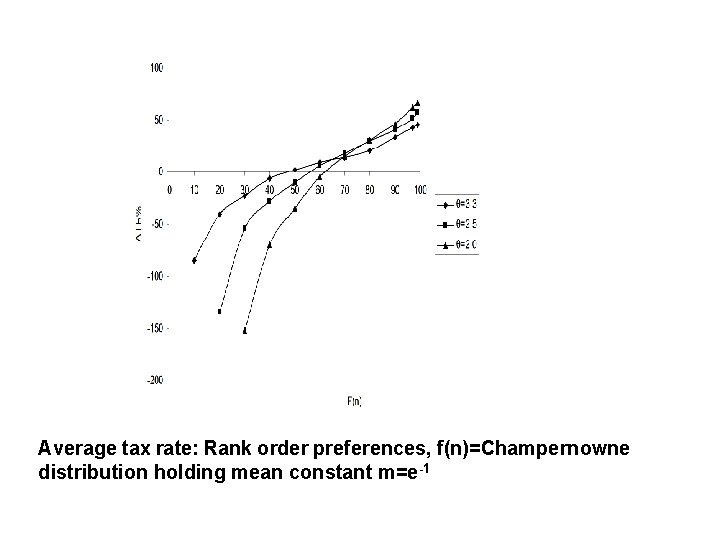
Average tax rate: Rank order preferences, f(n)=Champernowne distribution holding mean constant m=e-1

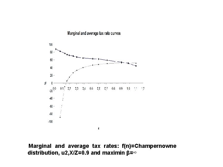
Marginal and average tax rates: f(n)=Champernowne distribution, u 2, X/Z=0. 9 and maximin β=∞

Marginal and average tax rates: f(n)=Champernowne distribution holding mean constant m=e-1 , θ =2. 5, , X/Z=0. 9 and utilitarian

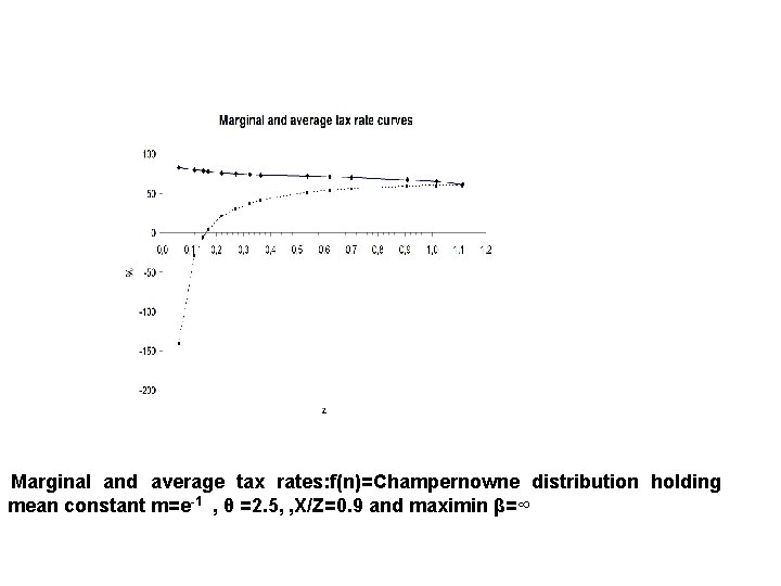
Marginal and average tax rates: f(n)=Champernowne distribution holding mean constant m=e-1 , θ =2. 5, , X/Z=0. 9 and maximin β=∞

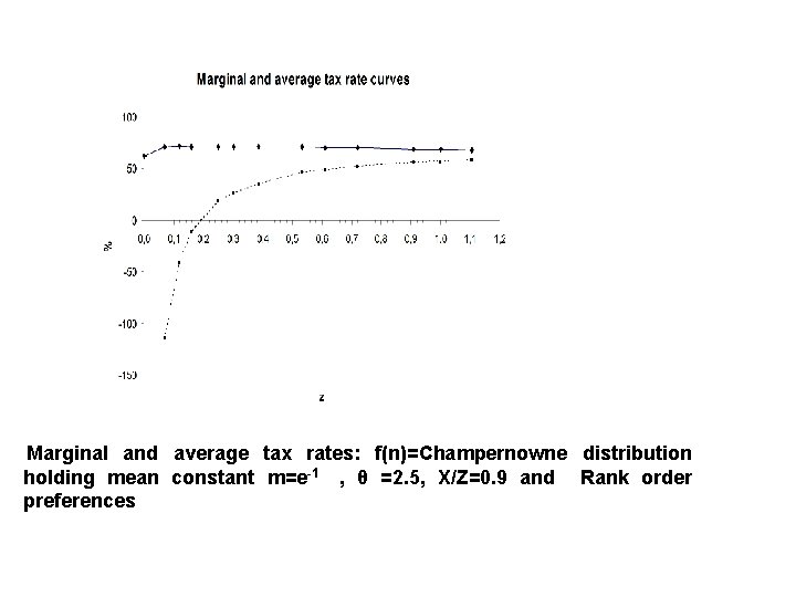
Marginal and average tax rates: f(n)=Champernowne distribution holding mean constant m=e-1 , θ =2. 5, X/Z=0. 9 and Rank order preferences

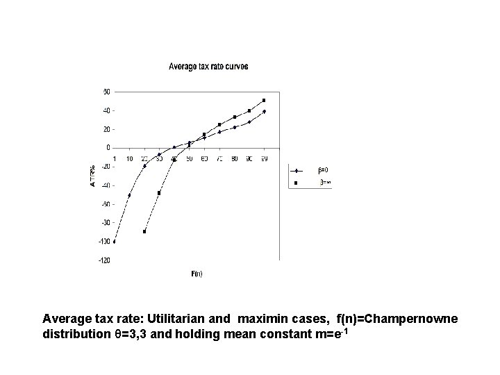
Average tax rate: Utilitarian and maximin cases, f(n)=Champernowne distribution θ=3, 3 and holding mean constant m=e-1

Concluding remarks • Numerical results suggest that the shift in tax burden seen in many countries cannot be justified in the Mirrlees model, which embodies conventional assumptions about inequality aversion and the trade of between equity and efficiency. • Figures show average tax rates decline among the bottom 70 percent when pre-tax inequality increases. • The main lesson for the tax policy is that we need more redistributive taxation, to tax the highest incomes more heavily.

Concluding remarks • So large has been the increase in the share of income going to the top 1 per cent that taxing them more heavily would only return them to the level of earnings they had a some decades ago. • It is hardly so that slightly higher taxes will drastically reduce labour supply among highearners. • But we will need to deal with tax avoidance and evasion, which is the more serious problem when taxing the rich more heavily