Optimal Execution of Coanalysis for Largescale Molecular Dynamics

Optimal Execution of Co-analysis for Large-scale Molecular Dynamics Simulations Preeti Malakar 1, Venkatram Vishwanath 1, Christopher Knight 1, Todd Munson 1, Michael E. Papka 12 1 Argonne National Laboratory 2 Northern Illinois University

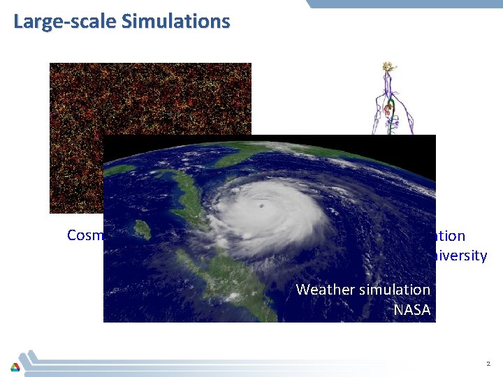
Large-scale Simulations Cosmological Simulation SDSS Blood Flow Simulation Randles Lab, Duke University Weather simulation NASA 2

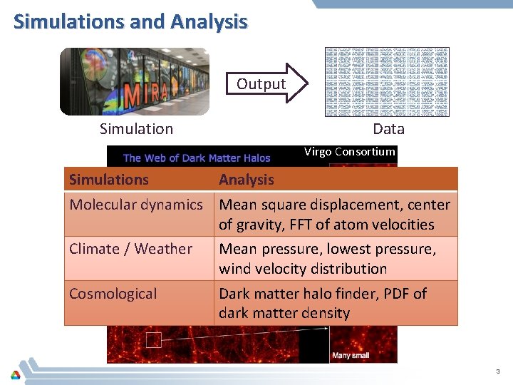
Simulations and Analysis Output Data Simulation Virgo Consortium Simulations Analysis Molecular dynamics Mean square displacement, center of gravity, FFT of atom velocities Climate / Weather Mean pressure, lowest pressure, wind velocity distribution Cosmological Dark matter halo finder, PDF of dark matter density 3

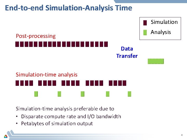
End-to-end Simulation-Analysis Time Simulation Analysis Post-processing Data Transfer Simulation-time analysis preferable due to • Disparate compute rate and I/O bandwidth • Petabytes of simulation output 4

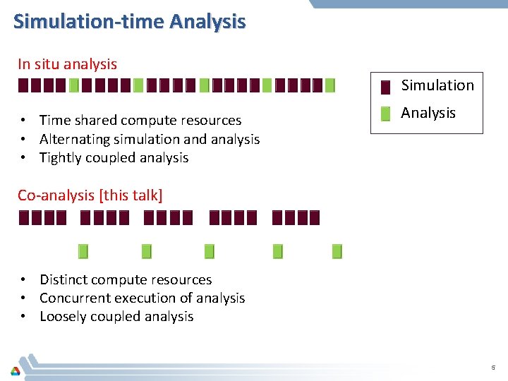
Simulation-time Analysis In situ analysis Simulation • Time shared compute resources • Alternating simulation and analysis • Tightly coupled analysis Analysis Co-analysis [this talk] • Distinct compute resources • Concurrent execution of analysis • Loosely coupled analysis 5

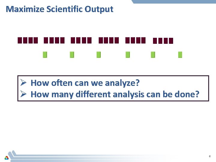
Maximize Scientific Output Ø How often can we analyze? Ø How many different analysis can be done? 6

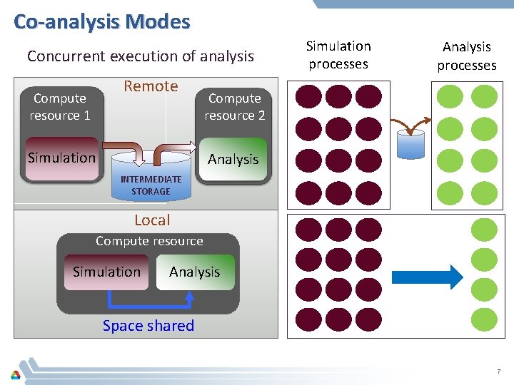
Co-analysis Modes Concurrent execution of analysis Compute resource 1 Remote Simulation processes Analysis processes Compute resource 2 Analysis INTERMEDIATE STORAGE Local Compute resource Simulation Analysis Space shared 7

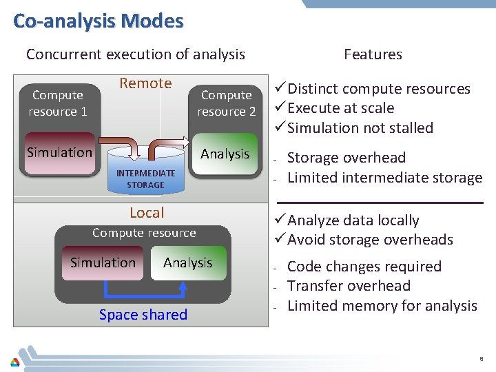
Co-analysis Modes Concurrent execution of analysis Compute resource 1 Remote Simulation Compute resource 2 ü Distinct compute resources ü Execute at scale ü Simulation not stalled Analysis - INTERMEDIATE STORAGE Local Compute resource Simulation Features Analysis - ü Analyze data locally ü Avoid storage overheads - Space shared Storage overhead Limited intermediate storage - Code changes required Transfer overhead Limited memory for analysis 8

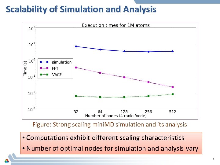
Scalability of Simulation and Analysis Figure: Strong scaling mini. MD simulation and its analysis • Computations exhibit different scaling characteristics • Number of optimal nodes for simulation and analysis vary 9

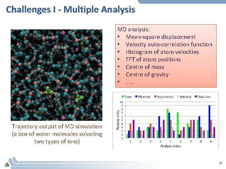
Challenges I - Multiple Analysis MD analysis: • Mean-square displacement • Velocity auto-correlation function • Histogram of atom velocities • FFT of atom positions • Centre of mass • Centre of gravity • . . . Trajectory output of MD simulation (a box of water molecules solvating two types of ions) 10

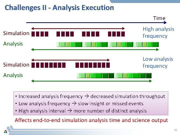
Challenges II - Analysis Execution Time Simulation High analysis frequency Analysis Simulation Low analysis frequency Analysis • Increased analysis frequency decreased simulation throughput • Low analysis frequency slow insight or missed events • High analysis interval more number of distinct analysis Affects end-to-end simulation analysis time and science output 11

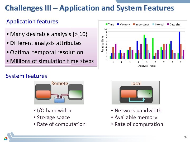
Challenges III – Application and System Features Application features • Many desirable analysis (> 10) • Different analysis attributes • Optimal temporal resolution • Millions of simulation time steps System features Remote Local • I/O bandwidth • Storage space • Rate of computation • Network bandwidth • Available memory • Rate of computation 12

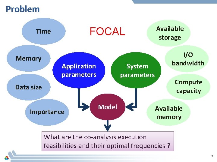
Problem FOCAL Time Memory Application parameters Available storage I/O bandwidth System parameters Compute capacity Data size Importance Model Available memory What are the co-analysis execution feasibilities and their optimal frequencies ? 13

Outline Ø FOCAL (Framework for Optimizing Co-analysis Executions) Ø Remote model Ø Local model Ø Application case study Ø Experiments and Results Ø Conclusions 14

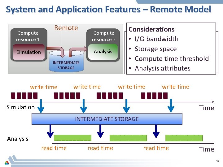
System and Application Features – Remote Model Compute resource 1 Remote Compute resource 2 Analysis Simulation INTERMEDIATE STORAGE write time Simulation Analysis Considerations • I/O bandwidth • Storage space • Compute time threshold • Analysis attributes write time Time Simulation INTERMEDIATE STORAGE Analysis read time Time 15

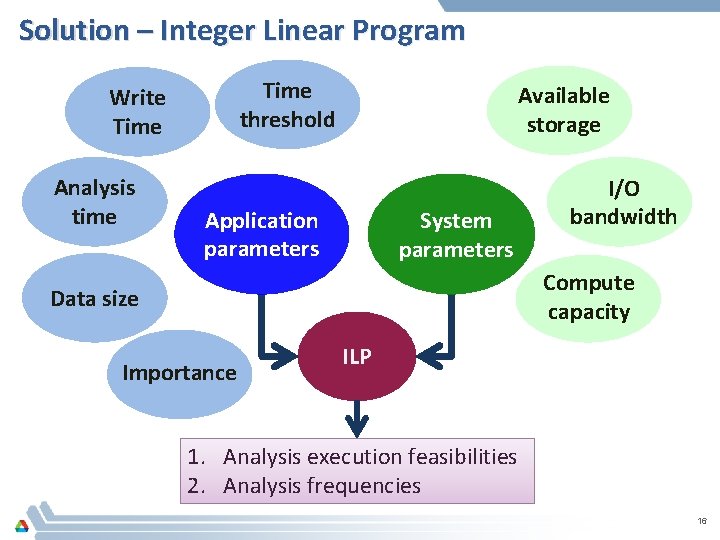
Solution – Integer Linear Program Time threshold Write Time Analysis time Available storage Application parameters System parameters I/O bandwidth Compute capacity Data size Importance ILP 1. Analysis execution feasibilities 2. Analysis frequencies 16

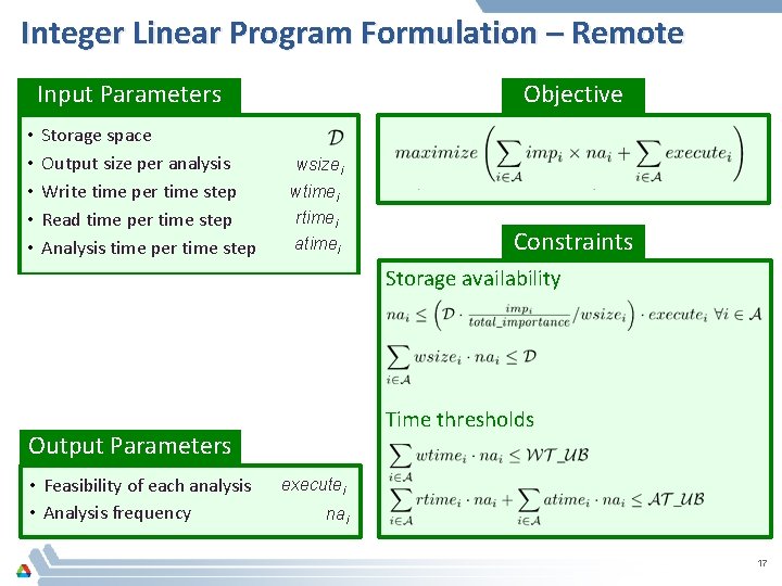
Integer Linear Program Formulation – Remote Input Parameters • • • Storage space Output size per analysis Write time per time step Read time per time step Analysis time per time step Objective wsizei wtimei rtimei atimei Set of analyses impi Importance of analysis Upper bound on write time WT_UB Upper bound on analysis time AT_UB Storage availability Time thresholds Output Parameters • Feasibility of each analysis • Analysis frequency Constraints executei nai 17

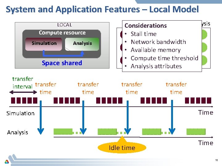
System and Application Features – Local Model LOCAL Compute resource Simulation Analysis Space shared transfer interval transfer time Simulation Analysis Considerations • Stall time • Network bandwidth • Available memory • Compute time threshold • Analysis attributes transfer time Time Simulation Analysis Idle time Time 18

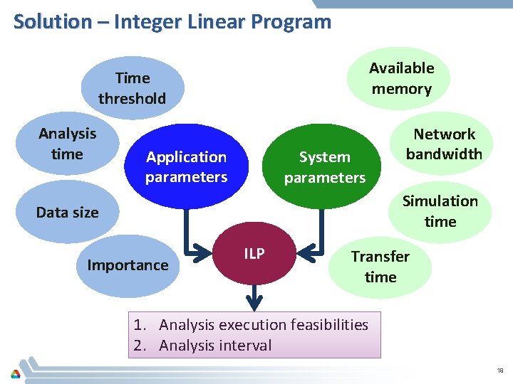
Solution – Integer Linear Program Available memory Time threshold Analysis time Application parameters System parameters Network bandwidth Simulation time Data size Importance ILP Transfer time 1. Analysis execution feasibilities 2. Analysis interval 19

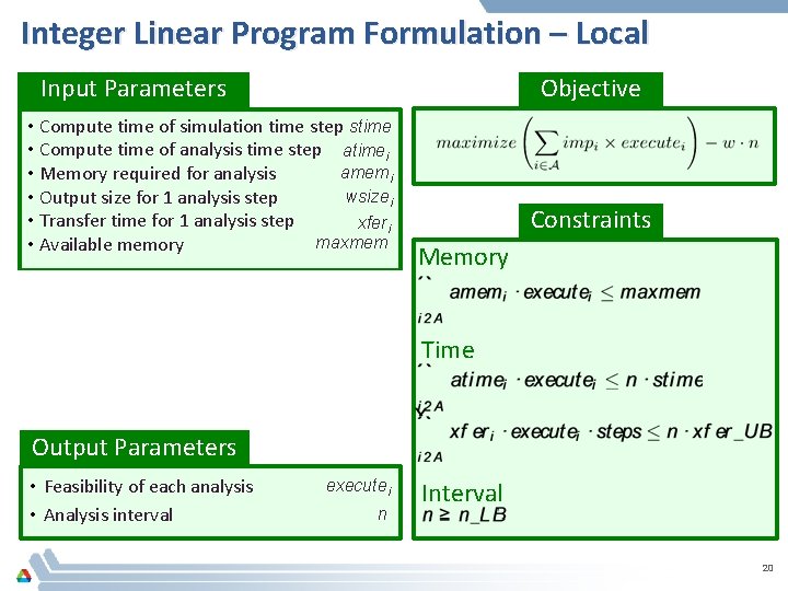
Integer Linear Program Formulation – Local Input Parameters Objective • Compute time of simulation time step stime • Compute time of analysis time step atimei amemi • Memory required for analysis wsizei • Output size for 1 analysis step • Transfer time for 1 analysis step xferi maxmem • Available memory • Set of analyses • Simulation steps • Importance of analysis • Upper bound on transfer time • Lower bound on analysis interval Constraints Memory steps impi xfer_UB n_UB Time executei Interval Output Parameters • Feasibility of each analysis • Analysis interval n 20

Outline Ø FOCAL (Framework for Optimizing Co-analysis Executions) Ø Remote model Ø Local model Ø Application case study Ø Experiments and Results Ø Conclusions 21

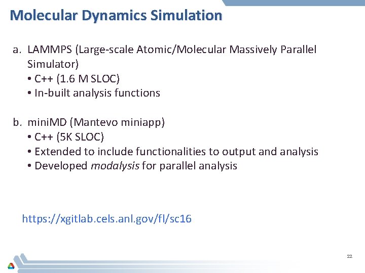
Molecular Dynamics Simulation a. LAMMPS (Large-scale Atomic/Molecular Massively Parallel Simulator) • C++ (1. 6 M SLOC) • In-built analysis functions b. mini. MD (Mantevo miniapp) • C++ (5 K SLOC) • Extended to include functionalities to output and analysis • Developed modalysis for parallel analysis https: //xgitlab. cels. anl. gov/fl/sc 16 22

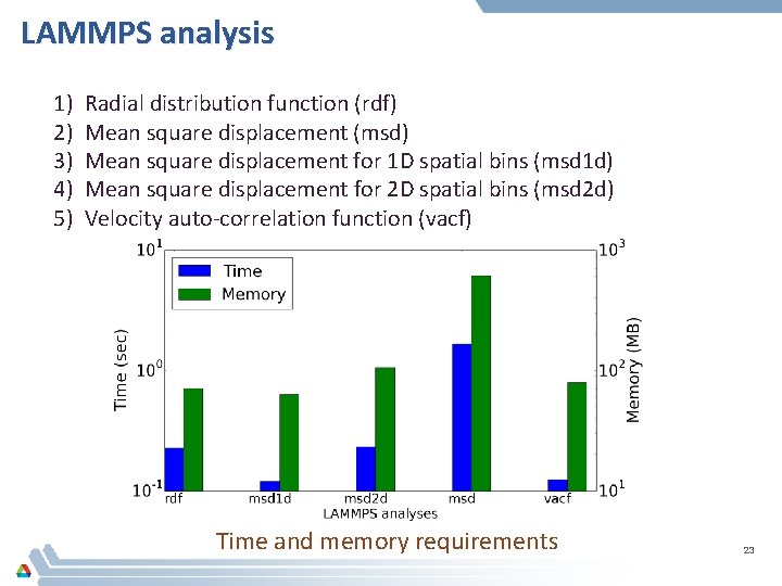
LAMMPS analysis 1) 2) 3) 4) 5) Radial distribution function (rdf) Mean square displacement (msd) Mean square displacement for 1 D spatial bins (msd 1 d) Mean square displacement for 2 D spatial bins (msd 2 d) Velocity auto-correlation function (vacf) Time and memory requirements 23

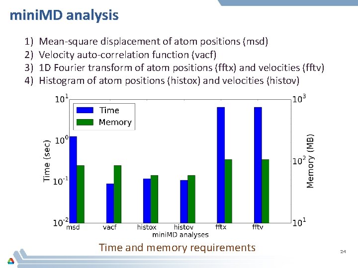
mini. MD analysis 1) 2) 3) 4) Mean-square displacement of atom positions (msd) Velocity auto-correlation function (vacf) 1 D Fourier transform of atom positions (fftx) and velocities (fftv) Histogram of atom positions (histox) and velocities (histov) Time and memory requirements 24

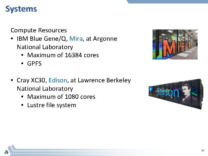
Systems Compute Resources • IBM Blue Gene/Q, Mira, at Argonne National Laboratory • Maximum of 16384 cores • GPFS • Cray XC 30, Edison, at Lawrence Berkeley National Laboratory • Maximum of 1080 cores • Lustre file system 25

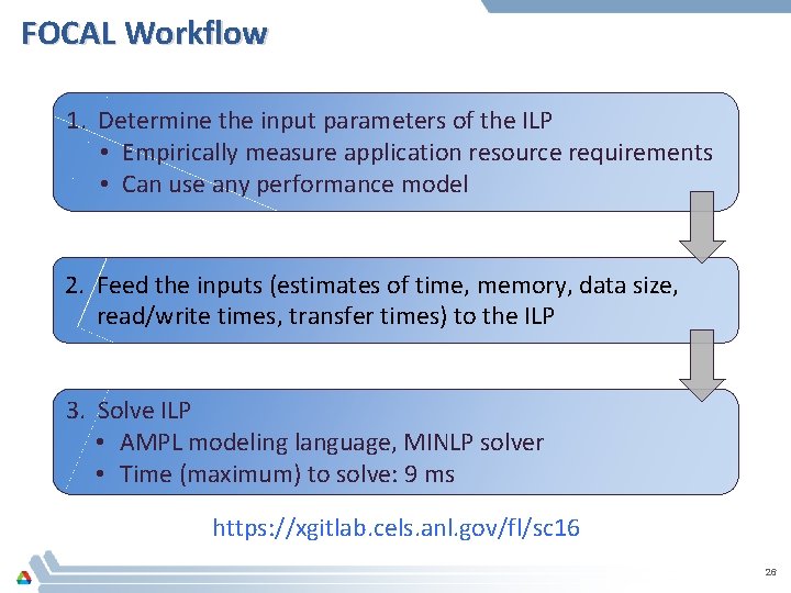
FOCAL Workflow 1. Determine the input parameters of the ILP • Empirically measure application resource requirements • Can use any performance model 2. Feed the inputs (estimates of time, memory, data size, read/write times, transfer times) to the ILP 3. Solve ILP • AMPL modeling language, MINLP solver • Time (maximum) to solve: 9 ms https: //xgitlab. cels. anl. gov/fl/sc 16 26

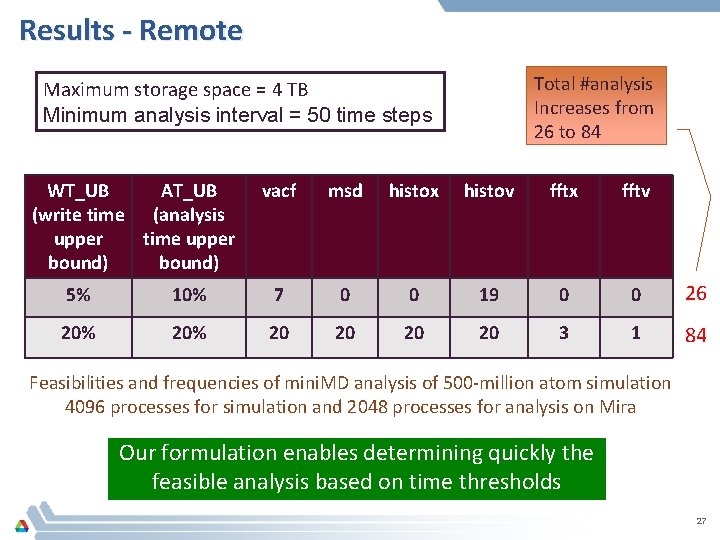
Results - Remote Total #analysis Increases from 26 to 84 Maximum storage space = 4 TB Minimum analysis interval = 50 time steps WT_UB AT_UB (write time (analysis upper time upper bound) vacf msd histox histov fftx fftv 5% 10% 7 0 0 19 0 0 26 20% 20 20 3 1 84 Feasibilities and frequencies of mini. MD analysis of 500 -million atom simulation 4096 processes for simulation and 2048 processes for analysis on Mira Our formulation enables determining quickly the feasible analysis based on time thresholds 27

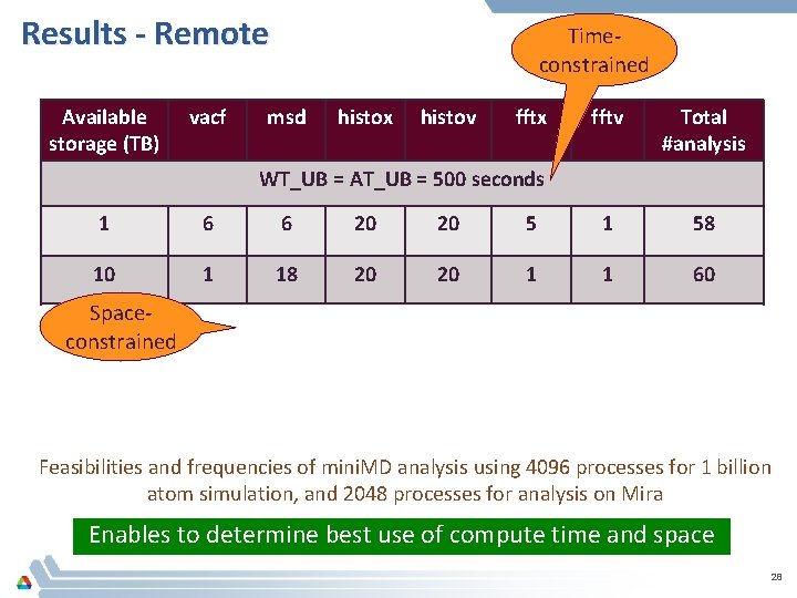
Results - Remote Available storage (TB) vacf Timeconstrained msd histox histov fftx fftv Total #analysis WT_UB = AT_UB = 500 seconds 1 6 6 20 20 5 1 58 10 1 18 20 20 1 1 60 Spaceconstrained 1 10 WT_UB = AT_UB = 1000 seconds 6 5 20 20 20 11 82 20 20 13 1 94 Feasibilities and frequencies of mini. MD analysis using 4096 processes for 1 billion atom simulation, and 2048 processes for analysis on Mira Enables to determine best use of compute time and space 28

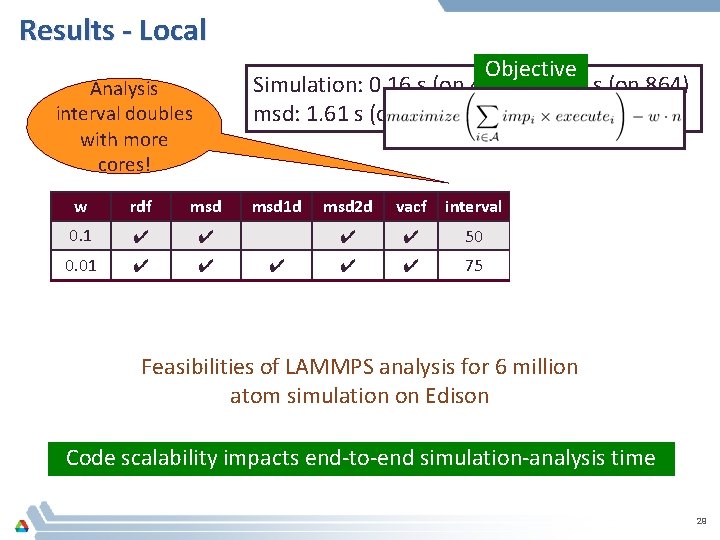
Results - Local Objective Simulation: 0. 16 s (on 432) to 0. 07 s (on 864) msd: 1. 61 s (on 144) to 1. 29 s (on 216) Analysis interval doubles with more cores! w rdf msd 0. 1 ✔ ✔ 0. 01 ✔ ✔ 0. 1 ✔ 0. 01 ✔ ✔ msd 1 d ✔ ✔ msd 2 d vacf interval #processes ✔ ✔ 50 432 (simulation) ✔ ✔ 75 144 (analysis) ✔ ✔ 58 864 (simulation) ✔ ✔ 172 216 (analysis) Feasibilities of LAMMPS analysis for 6 million atom simulation on Edison Code scalability impacts end-to-end simulation-analysis time 29

Conclusions • Formulated remote and local co-analysis as ILP • Consider system and application features to maximize scientific throughput • FOCAL provides useful recommendations • Feasible analysis and optimal analysis frequencies • Impact of more storage and more cores for analysis Future work • Extend to other co-analysis execution modes • Impact of code scalabilities 30

Acknowledgements • Argonne Leadership Computing Facility • National Energy Research Scientific Computing Centre This research has been funded in part and used resources of the Argonne Leadership Computing Facility at Argonne National Laboratory, which is supported by the Office of Science of the U. S. Department of Energy under contract DE-AC 02 -06 CH 11357. This work was supported in part by the DOE Office of Science, Advanced Scientific Computing Research, under award number 57 L 38, 57 L 32, 57 K 07 and 57 K 50. 31

Thank You! https: //xgitlab. cels. anl. gov/fl/sc 16 pmalakar@anl. gov 32