Optimal allocation and processing time decisions on nonidentical

Optimal allocation and processing time decisions on non-identical parallel CNC machines: e-constraint approach Seçil Sözüer 1

Agenda 1 -) 2 -) 3 -) 4 -) 5 -) 6 -) 7 -) Introduction Problem Defn. Single machine subproblem (Pm ) Cost lower bounds for a partial schedule (for B&B and BS) Initial solution (IS) (a heuristic for finding IS for B&B) B&B algorithm (exact algorithm) Beam search algorithm (BS) (if B&B: not computationally efficient) 8 -) Improvement search heuristic (ISH) (improves any given feasible schedule) 9 -) Recovering beam search (RBS) 10 -) Computational results 2

1. Introduction Turning (metal cutting) operation on non-identical parallel CNC machines � Controllable processing times in practice (attaining small proc. time by cutting speed or feed rate � Decide on ◦ Processing times of the jobs ◦ Machine / Job Allocation � Bicriteria Problem (Two objectives): COST and TIME � Total Manuf. Cost: � � ) & Makespan Converting Bicriteria Problem to Single Criterion Problem: e-constraint Approach: min. s. t. Makespan ≤ K (Upper Limit) Decision Maker: Interactively specify and modify K and analyze the influence of the changes on solutions 3

1. Introduction � � Controllable process. times: Pioneer: Vickson(1980) Problem: Total Process. Times & Total Weighted Compl. Time on a single machine Trick(1994): (Linear Process. Cost function) Nonidentical Parallel Mach. – NP-hard problem Problem: min. Total Process. Cost s. t. Makespan ≤ K (This paper considers nonlinear convex manuf. Cost Function) � Kayan and Aktürk(2005): Determining upper and lower bounds for process. Times and manuf. Cost function 4

2. Problem Definiton Parameters Each job is different in terms of its length and diameter, depth of cut, maximum allowable surface roughness, and its cutting tool type. Each job must be performed on a single machine without preemption is a convex fnc and minimized at N: M: number of jobs, card( J )= N number of machines m=1. . M Each machine is different in terms of its maximum applicable cutting power Hm, and its unit operating cost, Cm ($/minute). Operating Cost + Tooling Cost 5

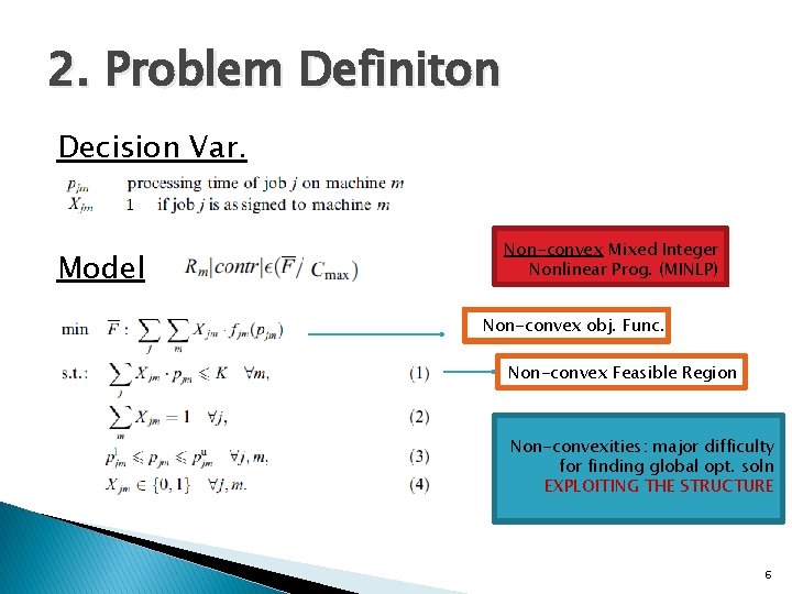
2. Problem Definiton Decision Var. Model Non-convex Mixed Integer Nonlinear Prog. (MINLP) Non-convex obj. Func. Non-convex Feasible Region Non-convexities: major difficulty for finding global opt. soln EXPLOITING THE STRUCTURE 6

3. Single Machine Subproblem (Pm) � With given Xjm (mach/job allocation), we can find optimal pjm by solving Pm for each machine m: Non-linear convex obj. func. Jm : set of jobs assigned to machine m. Convex Feasible Region Pm is convex. Hence local opt = global opt. Lemma 1 is sufficient for opt. is the Lagr. Dual var. for the makespan constraint (5). ≤ 0 since fjm is non-increasing on the interval (6) For the Lemma 1 proof: replace (6) and use KKT - CS Conditions 7

3. Single Machine Subproblem (Pm) Immediate extension of Lemma 1 to the non-ident. Parallel machine 8

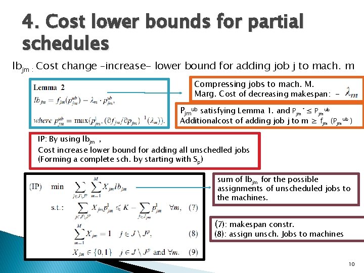
4. Cost lower bounds for partial schedules � � � � Sp : partial schedule Jp : subset of jobs assigned to machines Jmp : subset of jobs assigned to machine m optimal pjm decisions were made by solving the Pm We assume that when we add an unscheduled job to Sp, processing times of previously scheduled jobs may change, but the machine/job assignments in Sp stay the same. Adding an unscheduled job j to machine m does not violate the makespan constraint (1): hence The processing time decisions for the jobs in Jp were made previously by solving the Pm for each machine m, we have at hand the optimal dual price for each m. 9

4. Cost lower bounds for partial schedules lbjm : Cost change –increase- lower bound for adding job j to mach. m Compressing jobs to mach. M. Marg. Cost of decreasing makespan: Pjmub satisfying Lemma 1. and Pjm* ≤ Pjmub Additionalcost of adding job j to m ≥ fjm (Pjmub ) IP: By using lbjm , Cost increase lower bound for adding all unschedled jobs (Forming a complete sch. by starting with Sp) sum of lbjm for the possible assignments of unscheduled jobs to the machines. (7): makespan constr. (8): assign unsch. Jobs to machines 10

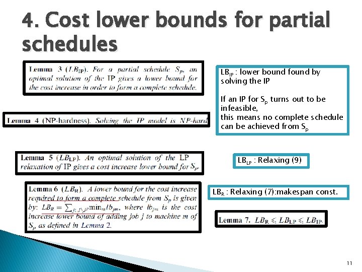
4. Cost lower bounds for partial schedules LBIP : lower bound found by solving the IP If an IP for Sp turns out to be infeasible, this means no complete schedule can be achieved from Sp LBLP : Relaxing (9) LBR : Relaxing (7): makespan const. 11

5. Initial Soln (IS) � IS: will be ub soln. For B&B Scheduling min-cost job first ! Each iteration: Adds a new job to schedule by choosing the best machine (that will give min. cost increase) Performance: N x M : iteration 12

6. B&B Algorithm � � � q The major difficulty in a B&B algorithm for a non-convex MINLP problem : computing a lb at a node of a B&B tree Each node: partial schedule (level 0: all jobs: unscheduled) (level k: jobs (j 1, . . . jk) : scheduled) For eah node, we find the opt. Cost and opt pjm by Pm (level N: all jobs: scheduled) Reducing the size of tree: Pruned by Infeasiblity? If feasible, solve Pm. Find a lb LBP ; LBIP or LBLP or LBR : Prune by inf? LBC = LBP + FP LB for complete sch. achievable from node q Cost incr. lb of the node Cost of the partial sch. If LBC ≥ UBC , Then Prune by Optimality Cost upperbound: initally found by IS, (then updated if we find a feas. complete sched) 13

6. B&B Algorithm Modified depth first search: Selects the one with minimum lb as new parent node 14

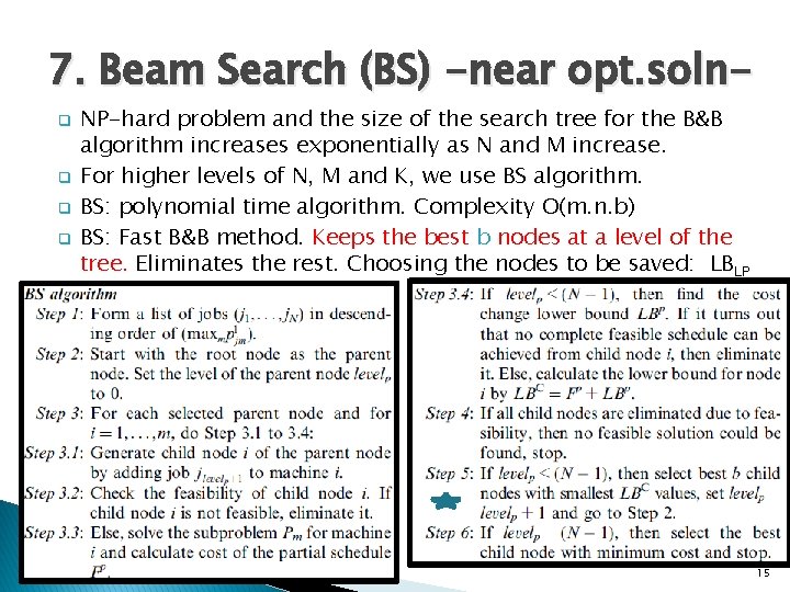
7. Beam Search (BS) -near opt. solnq q NP-hard problem and the size of the search tree for the B&B algorithm increases exponentially as N and M increase. For higher levels of N, M and K, we use BS algorithm. BS: polynomial time algorithm. Complexity O(m. n. b) BS: Fast B&B method. Keeps the best b nodes at a level of the tree. Eliminates the rest. Choosing the nodes to be saved: LBLP 15

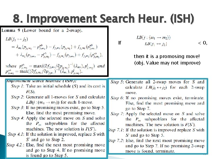
8. Improvement Search Heur. (ISH) Starts with an initial schedule which satisfies the optimality condition in Corollary 1 so that we assume the Pm is solved for each machine m. (We have at hand the optimal dual price for each m. ) � Define two moves to describe the neighborhood of a solution. 1 -move : move a job j from its current machine m 1 to another machine m 2 2 -swap : exchange job j 1 on machine m 1 with another job j 2 on machine m 2. � Cost of job j in m 1 Cost change lb by expanding proc. Times of the remaining jobs Adding job j to m 2 Removing job j from m 1 16

8. Improvement Search Heur. (ISH) If < 0, then it is a promosing move! (obj. Value may not improve) 17

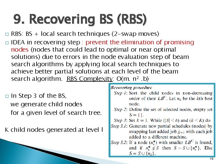
9. Recovering BS (RBS) � � � RBS: BS + local search techniques (2 -swap moves) IDEA in recovering step : prevent the elimination of promising nodes (nodes that could lead to optimal or near optimal solutions) due to errors in the node evaluation step of beam search algorithms by applying local search techniques to achieve better partial solutions at each level of the beam search algorithm. RBS Complexity: O(m. n 2. b) In Step 3 of the BS, we generate child nodes for a given level of search tree. K child nodes generated at level l 18

10. Computational Results Selecting K: makespan limit (In order to see the effect of K, solving each replication of the problem for 5 different levels of K. ) � To find proper K: � First, solving the makespan minimization problem for each replication for fixed processing times case where for each j and m. : NP-HARD � Polyn. -Time Algorithm: finding a feasible makespan level K: KDJ � K = k x KDJ k = 0. 6, 0. 8, 1, 1. 2, 1. 4 � Solving each B&B : with LBIP , LBLP, LBR � If B&B finds opt. soln: Solving the problem with BS and RBS (LB LP) � kn � 19

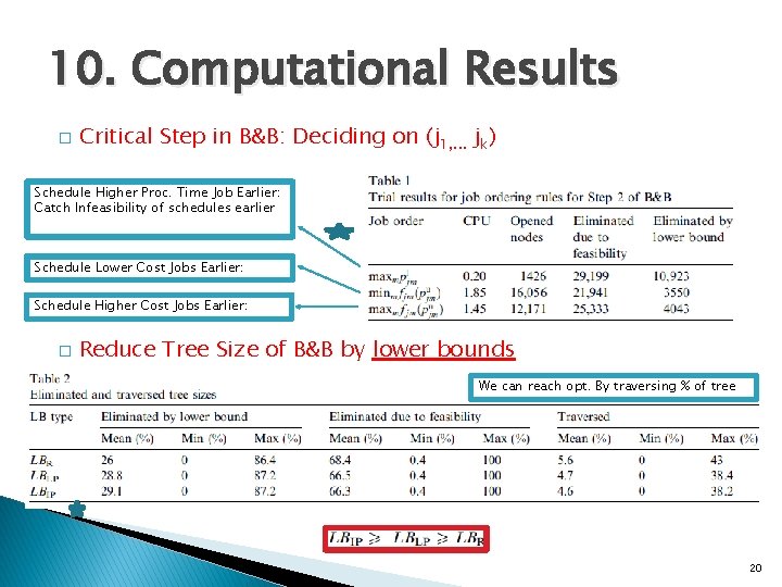
10. Computational Results � Critical Step in B&B: Deciding on (j 1, . . . jk) Schedule Higher Proc. Time Job Earlier: Catch Infeasibility of schedules earlier Schedule Lower Cost Jobs Earlier: Schedule Higher Cost Jobs Earlier: � Reduce Tree Size of B&B by lower bounds We can reach opt. By traversing % of tree 20

10. Computational Results � The effect of Increasing N and M on running time of B&B Big Gap btwn «Min» and «Max» for each lower bounding method due to different K levels Calculating LBR is faster. As N and M increase, the CPU time required by LBR approaches to LBLP, so we may expect to see that LBLP will have shorter CPU times for larger problem sizes. . If we check the CPU time ratio LBR / LBIP, we observe that as N is increased, performance of the LBR gets closer to the performance of LBIP, but as M is increased, we observe the opposite. This is due to the fact that computing LBIP is itself an NP-hard problem and requires much more time when M is increased. 21

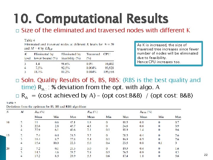
10. Computational Results � Size of the eliminated and traversed nodes with different K As K is increased, the size of traversed tree increases since fewer number of nodes will be eliminated due to feasibility. Hence CPU increases too. � � Soln. Quality Results of IS, BS, RBS: (RBS is the best quality and time) RA : : % deviation from the opt. with algo. A RA = (cost achieved by A) – (opt cost: B&B) / (opt cost: B&B) 22

10. Computational Results � ISH achieves a significant improvement for all 3 cases RA+ISH = starting soln with algo A and improve through ISH Comparing Table 5 and 6 23

10. Computational Results � � Soln quality of BS and ISH improves as K is increased Hence, if B&B: not efficient, BS and ISH can achieve soln closer to optimum. This is due to the shape of manuf. Cost func. When K is increased, we have higher process. Time: flatter manuf. Cost func. 24

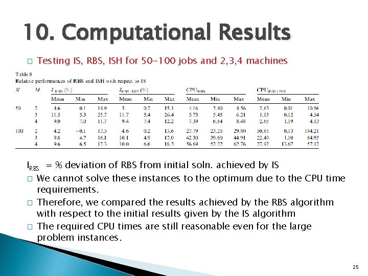
10. Computational Results � Testing IS, RBS, ISH for 50 -100 jobs and 2, 3, 4 machines IRBS = % deviation of RBS from initial soln. achieved by IS � We cannot solve these instances to the optimum due to the CPU time requirements. � Therefore, we compared the results achieved by the RBS algorithm with respect to the initial results given by the IS algorithm � The required CPU times are still reasonable even for the large problem instances. 25

10. Computational Results � � � Our computational results show that B&B can solve the problems by just traversing the 5% of the maximal possible (Slide 20)-Table-2 B&B tree size and the proposed lower bounding methods can eliminate up to 80% of the search tree. (Table 2) For the cases where B&B is not computationally efficient, our BS and improvement search algorithms achieved solutions within 1% of the optimum on the average in a very short computation time. 26