Optical surveys sensors for the upgrade Adrian Bevan

Optical surveys: sensors for the upgrade Adrian Bevan, Karen Hayrapetyan, Camillia Messiouni 1

Overview • ROOT is too slow to process large data sets from our smartscope; so have adopted an analysis procedure using Matlab. • Fast • Felxible • Easy to use • . . but requires some of us to learn a new tool Mechanicals are flat Sensors are bowed; either convex or concave depending on vendor/process details 2

QA model • Collect data in a grid with a finite spacing between measurement points. – Time: 15 min for a scan in (x, y) steps of 500 um • Plot and fit the data points with a plane. – Time: seconds (gave up on ROOT) • Histogram the residuals about the mean defined by the plane; use spread as QA metric. – Acquisition with the OGP software and post processing by Matlab is quick enough that we _can_ assay all sensors passing through our lab before electrical testing. – i. e. can quickly pass/fail sensors out of QA bound of 200 um bowing. 3

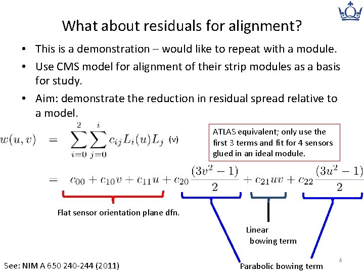
What about residuals for alignment? • This is a demonstration – would like to repeat with a module. • Use CMS model for alignment of their strip modules as a basis for study. • Aim: demonstrate the reduction in residual spread relative to a model. (v) ATLAS equivalent; only use the first 3 terms and fit for 4 sensors glued in an ideal module. Flat sensor orientation plane dfn. Linear bowing term See: NIM A 650 240 -244 (2011) Parabolic bowing term 4

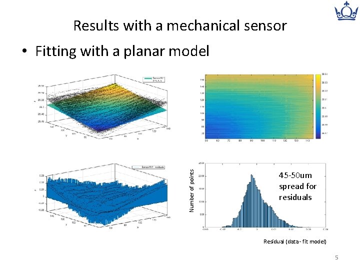
Results with a mechanical sensor Number of points • Fitting with a planar model 45 -50 um spread for residuals Residual (data - fit model) 5

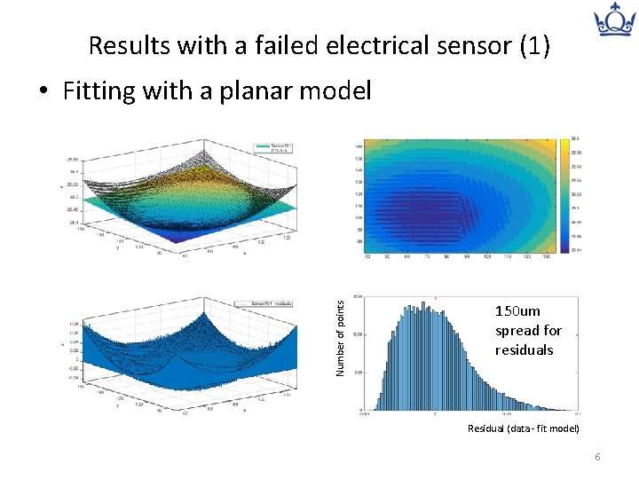
Results with a failed electrical sensor (1) Number of points • Fitting with a planar model 150 um spread for residuals Residual (data - fit model) 6

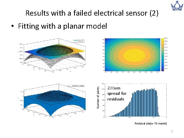
Results with a failed electrical sensor (2) Number of points • Fitting with a planar model 200 um spread for residuals Residual (data - fit model) 7

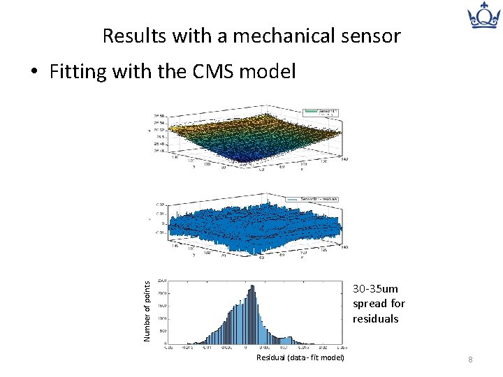
Results with a mechanical sensor • Fitting with the CMS model Number of points 30 -35 um spread for residuals Residual (data - fit model) 8

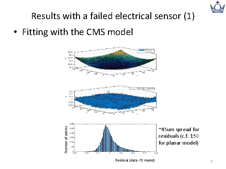
Results with a failed electrical sensor (1) • Fitting with the CMS model Number of points ~45 um spread for residuals (c. f. 150 for planar model) Residual (data - fit model) 9

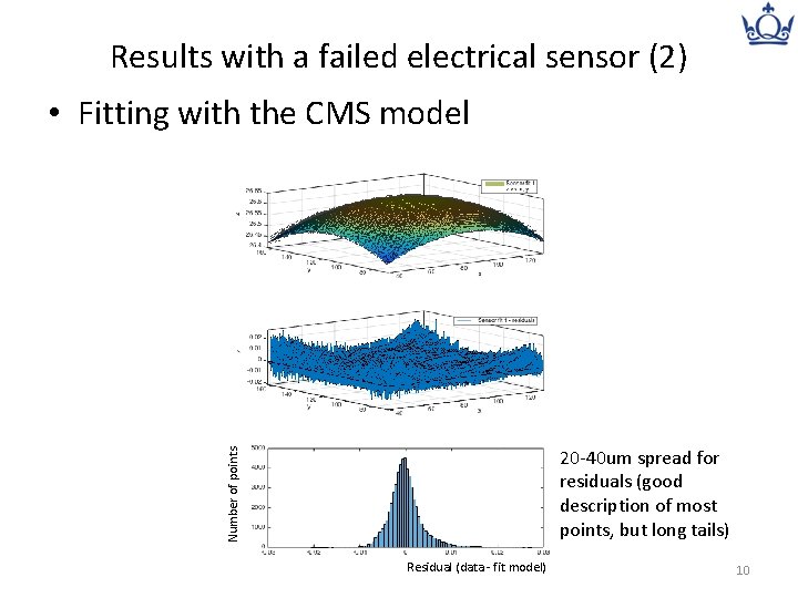
Results with a failed electrical sensor (2) • Fitting with the CMS model Number of points 20 -40 um spread for residuals (good description of most points, but long tails) Residual (data - fit model) 10

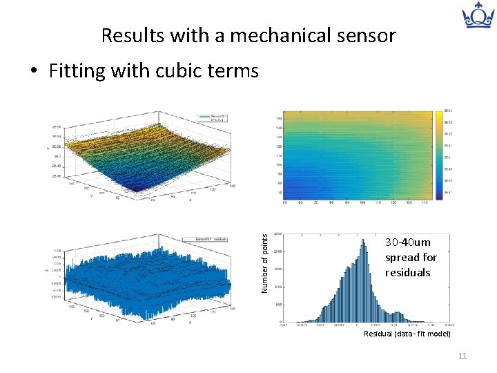
Results with a mechanical sensor Number of points • Fitting with cubic terms 30 -40 um spread for residuals Residual (data - fit model) 11

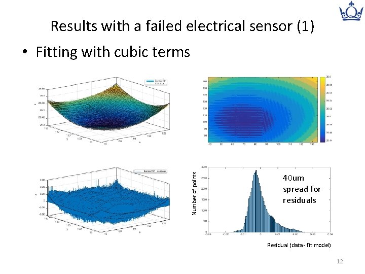
Results with a failed electrical sensor (1) Number of points • Fitting with cubic terms 40 um spread for residuals Residual (data - fit model) 12

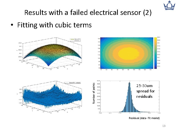
Results with a failed electrical sensor (2) Number of points • Fitting with cubic terms 25 -30 um spread for residuals Residual (data - fit model) 13

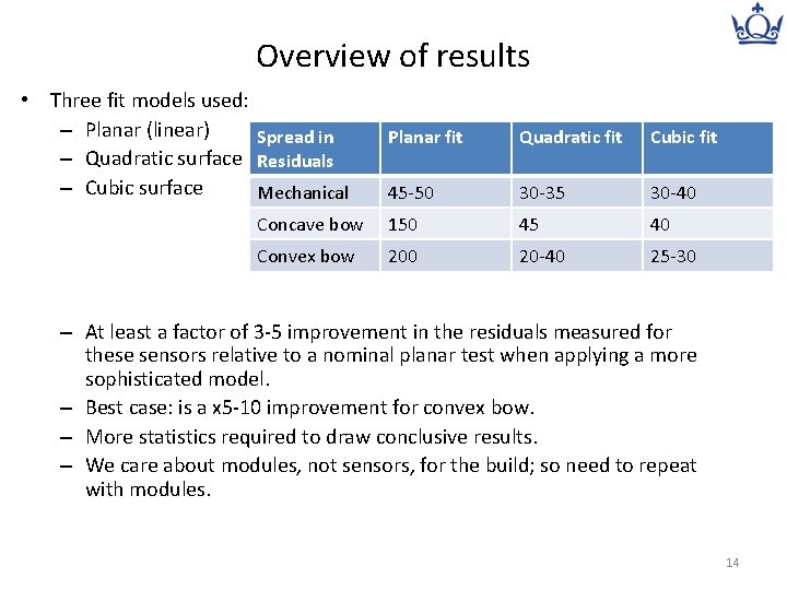
Overview of results • Three fit models used: – Planar (linear) Spread in – Quadratic surface Residuals – Cubic surface Mechanical Planar fit Quadratic fit Cubic fit 45 -50 30 -35 30 -40 Concave bow 150 45 40 Convex bow 200 20 -40 25 -30 – At least a factor of 3 -5 improvement in the residuals measured for these sensors relative to a nominal planar test when applying a more sophisticated model. – Best case: is a x 5 -10 improvement for convex bow. – More statistics required to draw conclusive results. – We care about modules, not sensors, for the build; so need to repeat with modules. 14

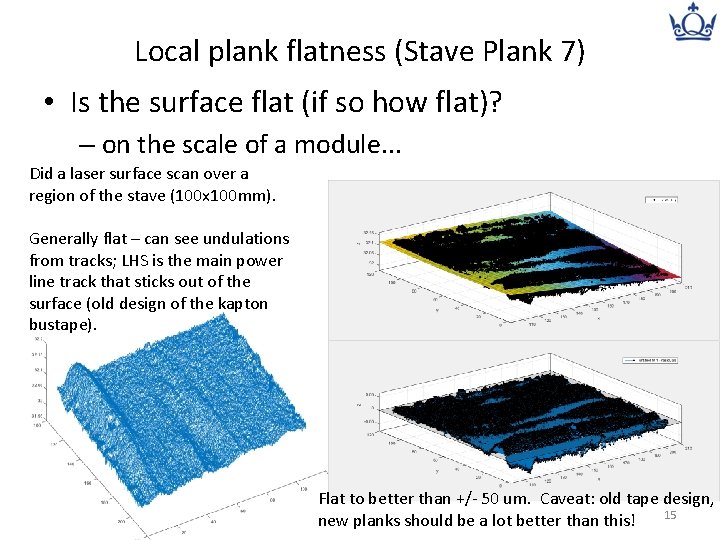
Local plank flatness (Stave Plank 7) • Is the surface flat (if so how flat)? – on the scale of a module. . . Did a laser surface scan over a region of the stave (100 x 100 mm). Generally flat – can see undulations from tracks; LHS is the main power line track that sticks out of the surface (old design of the kapton bustape). Flat to better than +/- 50 um. Caveat: old tape design, 15 new planks should be a lot better than this!

Summary • Can reduce the hypothetical position error by a significant factor: – x 3 -5 with these sensor tests. – Want to repeat with modules to quantify how this would affect the real items going into the SCT / pixel system. • Also plan to do cooling tests: exploring the possibility of having this as part of an ATLAS authorship task for a student. 16