Optical flow A tutorial of the paper G

Optical flow , A tutorial of the paper: G. Farneback , “Two-frame Motion Estimation based on Polynomial Expansion”, 13 th Scandinavian Conference, SCIA 2003 Halmstad, Sweden, June 29 – July 2, 2003. KH Wong Optical Flow v. 5 a (beta) 1

Introduction • Optical flow : Based on two frames sampled at different slight different time, find the change of position of each pixel in the first image to the second image. • Reference: • G. Farneback , “Two-frame Motion Estimation based on Polynomial Expansion”, 13 th Scandinavian Conference, SCIA 2003 Halmstad, Sweden, June 29 – July 2, 2003. Optical Flow v. 5 a 2

Problem definition and method • Problem: – Input: Two images – Output : motion vectors (v) and xx( c )? of each pixel in the first image. – The Farneback method [1] is fast and linear. • Method: – Step 1: Approximate the image using a polynomial – Step 2: Use the model of polynomial to approximate the motion for each pixel. Optical Flow v. 5 a 3

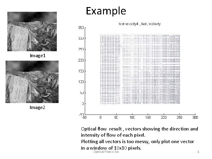
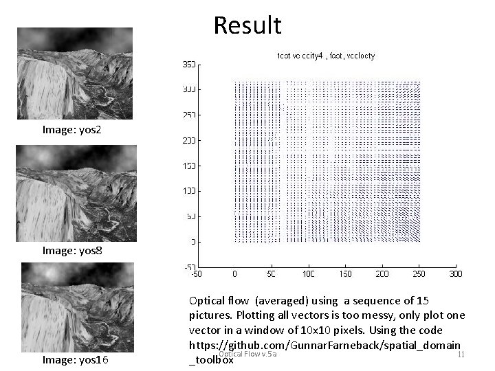
Example • Image 1 Image 2 Optical flow result , vectors showing the direction and intensity of flow of each pixel. Plotting all vectors is too messy, only plot one vector in a window of 10 x 10 pixels. Optical Flow v. 5 a 4

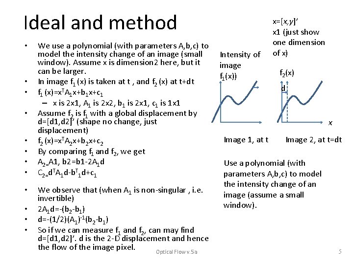
Ideal and method • • • We use a polynomial (with parameters A, b, c) to model the intensity change of an image (small window). Assume x is dimension 2 here, but it can be larger. In image f 1 (x) is taken at t , and f 2 (x) at t+dt f 1 (x)=x. TA 1 x+b 1 x+c 1 – x is 2 x 1, A 1 is 2 x 2, b 1 is 2 x 1, c 1 is 1 x 1 Assume f 2 is f 1 with a global displacement by d=[d 1, d 2]’ (shape no change, just displacement) f 2 (x)=x. TA 2 x+b 2 x+c 2 By comparing f 1 and f 2, we get A 2=A 1, b 2=b 1 -2 A 1 d C 2=d. TA 1 d-b. T 1 d+c 1 We observe that (when A 1 is non-singular , i. e. invertible) 2 A 1 d=-(b 2 -b 1) d=-(1/2)(A 1)-1(b 2 -b 1) So if we can measure f 1 and f 2, can may find d=[d 1, d 2]’. d is the 2 -D displacement and hence the flow of the image pixel. Optical Flow v. 5 a Intensity of image f 1(x)) x=[x, y]’ x 1 (just show one dimension of x) f 2(x) d x Image 1, at t Image 2, at t=dt Use a polynomial (with parameters A, b, c) to model the intensity change of an image (assume a small window). 5

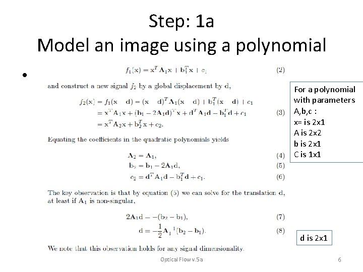
Step: 1 a Model an image using a polynomial • For a polynomial with parameters A, b, c : x= is 2 x 1 A is 2 x 2 b is 2 x 1 C is 1 x 1 d is 2 x 1 Optical Flow v. 5 a 6

Modeling images using polynomials • Read the Ph. D thesis • Orientation and Velocity, Estimation , Ph. D https: //www. facebook. com/download/33352 3813505207/farneback 99 -phd. pdf (page 22 the example) • and also the code make_Abc_fast. m in Code, https: //github. com/Gunnar. Farneback/spatial_ domain_toolbox • Optical Flow v. 5 a 7

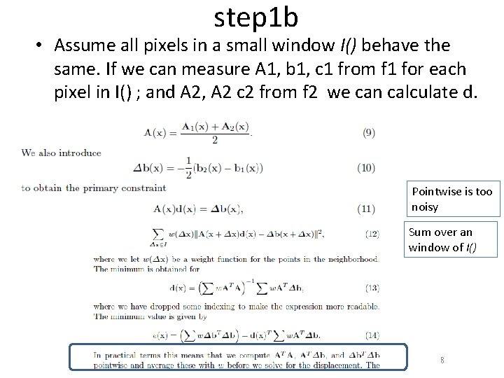
step 1 b • Assume all pixels in a small window I() behave the same. If we can measure A 1, b 1, c 1 from f 1 for each pixel in I() ; and A 2, A 2 c 2 from f 2 we can calculate d. Pointwise is too noisy Sum over an window of I() Optical Flow v. 5 a 8

Step 2 : find displacement d=[dx, dy]’ (=optical flow) • We assume d is not a constant over the window I(), but a function according to its position x, y based on affine transformation. Affine model of d 0 S is 2 x 8 ST is 8 x 2 p is 8 x 1 d is 2 x 1 wi= is 1 x 1 A , p , b can be measured. Put them in (19) and minimize (19), or set it to [0, 0]’. We can solve for p using (20), if p is found d can be found by (15) Optical Flow v. 5 a 9

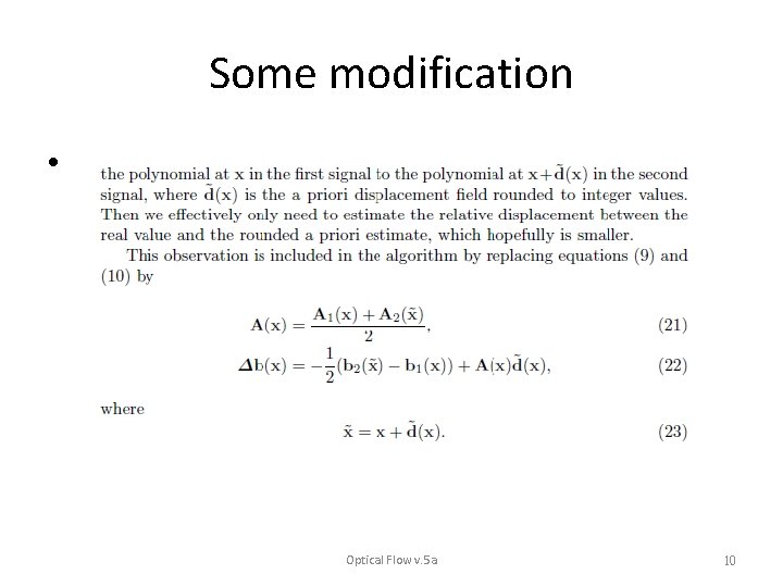
Some modification • Optical Flow v. 5 a 10

Result • Image: yos 2 Image: yos 8 Image: yos 16 Optical flow (averaged) using a sequence of 15 pictures. Plotting all vectors is too messy, only plot one vector in a window of 10 x 10 pixels. Using the code https: //github. com/Gunnar. Farneback/spatial_domain Optical Flow v. 5 a 11 _toolbox

Summary • Studied a linear method to find the optical flow based on two frames of image. Optical Flow v. 5 a 12

References 1) G. Farneback , “Two-frame Motion Estimation based on Polynomial Expansion”, 13 th Scandinavian Conference, SCIA 2003 Halmstad, Sweden, June 29 – July 2, 2003. 2) Publications of G. Farneback , http: //lmi. bwh. harvard. edu/papers/gunnar. html 3) G. Farneback , Spatial Domain Methods for 4) Orientation and Velocity, Estimation , Ph. D https: //www. facebook. com/download/333523813505207 /farneback 99 -phd. pdf 5) Code, https: //github. com/Gunnar. Farneback/spatial_domain_to olbox Optical Flow v. 5 a 13