Optical astronomical spectroscopy at the VLT Part 2

Optical astronomical spectroscopy at the VLT (Part 2) F. Pepe Observatoire de Genève

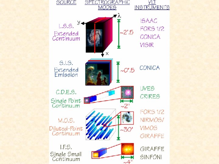
Course outline • • PART 1 - Principles of spectroscopy – Fundamental parameters – Overview of spectrometry methods PART 2 – ‘Modern’ spectrographs – ‘Simple’ spectroimager • – • FORS Echelle spectrographs • UVES • CRIRES PART 3 - Spectroscopy on the VLTs – – Multi-Object spectrographs (MOS) and Intergral-Field Units (IFU) and spectro-imagers • Giraffe • VIMOS • Sinfoni Future instruments • X-shooter • MUSE • ESPRESSO

Resolving power and resolution The objective translates angles into positions on the detector. Each position (pixel) of the detector ‘sees’ a given angle of the parallel (collimated) beam The collimated beam is never perfectly parallel, because either of the limited diameter of the beam, which produces diffraction df = 1. 22 l/D 1, or because of the finite slit, which produces and angular divergence d. Q = s/f 1. The angular divergence is translated into a distance dl = f 2 d. Q or dl = f 2 df on the CCD. This means that over this distances the wavelengths are mixed (cannot be separated angularly.

Resolving power and resolution Resolving power is the maximum spectral resolution which can be reached if the slit s = 0 and the angular divergence is limited by diffraction arising from the limited beam diameter. For a given Dispersion D we get the resolving power: Spectral resolution is the effective spectral resolution which is finally reached when assuming a finite slit s. For a given Dispersion D we get the spectral resolution:

Example of spectrographs Basic Parameters • Telescope diameter: DT • Source/seeing/slit: ssky • Collimated beam of the spectrograph: D 1 Other parameters: • Telescope focal length: f. T • Telescope F-number (focal ratio): FT = F = f. T/DT • Physical slit/fiber width: s = f. T x ssky • Collimator focal length: f 1 • Objective focal length: f 2

Grating spectrograph Focal ratios defined as Fi = fi / D i Camera Collimator

Example of simple spectrographs Spectral resolution: where

Example of ‘simple’ spectrographs Coralie@Euler: • Telescope diameter: DT = 1. 2 m • Source/seeing/slit: ssky = 1 arcsec • Collimated beam of the spectrograph: D 1 = 75 mm

Example of ‘simple’ spectrographs With prism: BK 7 (normal glass), t = 50 mm With grism: m = 1, r = 150 gr/mm, cosb=1

FORS@VLT

FORS@VLT

FORS@VLT

FORS@VLT

FORS: Filter mode

FORS: Grism mode • Grisms from 150 gr/mm to 1400 gr/mm • Spectroscopic modes – ‘slitless’ MOS mode (R is given by seeing) – Mask with up to 9 ‘long slits’ of 0. 3” x 6. 8’ – Up to 19 movable ‘slitlets’ of 0. 3” x 22. 5” – MOS-MXU: Laser-cut masks (any format) • Spectral resolution depends on grism dispersion and slit width in dispersion direction.

FORS: Grism mode Movable slilets (localized sourcess in ‘crowded fields) Long slit (extended sources, 1 -D image + spectrum)

FORS: MOS mode

FORS@VLT

FORS@VLT This image shows the first spectrum obtained of the comet 1995 Q 1. The spectral coverage extends from about 3650 Angstrom (left) to 4100 Angstrom (right) in the violet region. The spectrograph slit was oriented along the main tail at position angle ~ 145 degrees. The total slit length was 5. 6 arcminutes. The spectrum is typical for a comet at Comet Bradfield's current distance from the Sun (0. 5 A. U. , or about 75 million kilometres).

FORS: Spectral resolution • Telescope diameter: DT = 8. 2 m • Source/seeing/slit: ssky = 0. 3 arcsec • Collimated beam : D 1 = 125 mm With grism: m = 1, r = 1400 gr/mm, cosb=1

Example of ‘simple’ spectrographs • With single prisms resolution remains small • Possibility to increase dispersion by adding up several prisms • With gratings or grisms, the spectral resolution is up to several 1000 but still modest. • Other ‘tricks’ required

Echelle grating • Increase dispersion of the ordinary greating by increasing the difference between entrance and exit angle • The use in Littrow condition will make the mounting symmetric and maximize a + b, since a is set equal to b: a�= b • Use in blaze condition for maximum efficiency: Groove angle g�= b

Echelle grating From the grating equation we derive the dispersion law of an echelle grating: Example: R = 4 grating:

Characteristics of Echelle grating • High dispersion -> high resolution • Spectrum becomes VERY long and efficiency drops because of blaze function • Alternative: use at high order, e. g. m = 100 (r = 30 gr/mm) • -> Orders overlap spacially and must be separated (filtering, pre-dispersion or cross-dispersion) Free spectral range: Numbers of orders for full ‘octave’:

Multiple orders • Many orders to cover desired ll: Free spectral range Fl= l/m • Orders lie on top of each other: l(m) = l(n) (n/m) • Solution: – use narrow passband filter to isolate one order at a time – cross-disperse to fill detector with many orders at once Blaze condition fulfilled Cross dispersion may use prisms or low dispersion grating

Cross dispersion (prism, grating) -> Monochromatic image of the slit Main dispersion (echelle grating) ->

UVES@VLT

UVES@VLT

UVES@VLT

Coralie@Euler

UVES@VLT

UVES: Spectral format

UVES: Order separation

UVES: Spectral resolution • Telescope diameter: DT = 8. 2 m • Source/seeing/slit: ssky = 0. 3 arcsec • Collimated beam of the spectrograph: D 1 = 200 mm Echelle grating: R 4 -> tanb = 4, D 1 = 200 mm

UVES: Sampling and resolution

UVES: Image slicer ‘trick’ Long slit Image slicer Increase of efficiency at give R, or vice versa

UVES params

UVES: Efficiency

CRIRES@VLT

CRIRES@VLT Same as UVES, but: • For IR (l = 1 – 5. 4 µm) • Can use adaptive optics • Cryogenics needed • No cross-disperser. Only 1 order at a time! -> Pre-disperser

CRIRES@VLT, AO

CRIRES: Characteristics

CRIRES: Spectral format

CRIRES: Long slit

CRIRES@VLT Peculiarities of the IR domain: • Detector technology (no Si-CCDs, behavior less ‘ideal’ in terms of noise, flat-field stability, etc. ) • Thermal and sky back-ground -> remove e. g. by ‘nodding’ over long slit and put instrument ‘cold’ • Atmospheric absorption and emission features • Advantage: Use of adaptive optics to reduce slit width.

CRIRES@VLT