Opportunities for using AI methods in weather forecasting

Opportunities for using AI methods in weather forecasting at ECMWF Alan Geer Earth System Assimilation Section, Research Department Thanks to: Patricia de Rosnay, Peter Dueben, Peter Bauer, Leonhard Scheck (DWD/LMU), Elias Holm, Peter Lean, Massimo Bonavita, Marcin Chrust, Robin Hogan, Mohamed Dahoui, Lars Isaksen, Stephen English, Andy Brown © ECMWF June 3, 2021

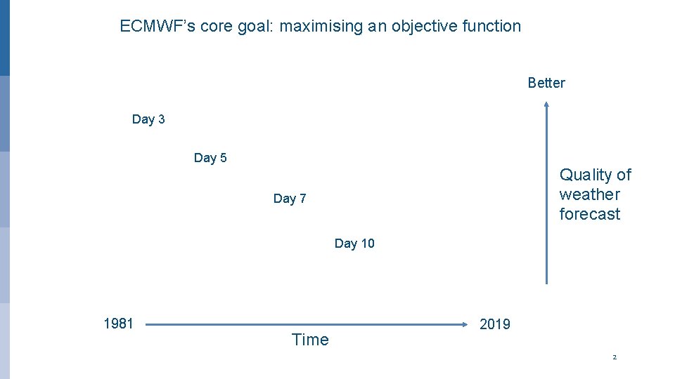
ECMWF’s core goal: maximising an objective function Better Day 3 Day 5 Quality of weather forecast Day 7 Day 10 1981 Time EUROPEAN CENTRE FOR MEDIUM-RANGE WEATHER FORECASTS 2019 2

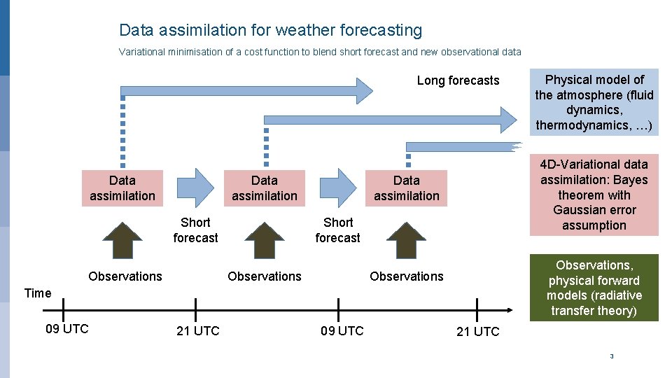
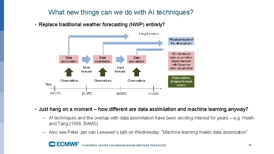
Data assimilation for weather forecasting Variational minimisation of a cost function to blend short forecast and new observational data Long forecasts Data assimilation Short forecast Observations 4 D-Variational data assimilation: Bayes theorem with Gaussian error assumption Data assimilation Observations, physical forward models (radiative transfer theory) Observations Time 09 UTC 21 UTC 09 UTC EUROPEAN CENTRE FOR MEDIUM-RANGE WEATHER FORECASTS Physical model of the atmosphere (fluid dynamics, thermodynamics, …) 21 UTC 3

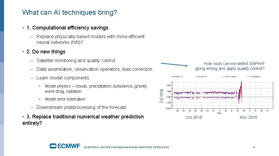
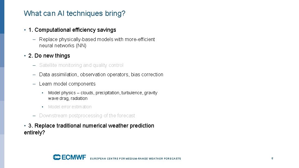
What can AI techniques bring? • 1. Computational efficiency savings – Replace physically-based models with more-efficient neural networks (NN)? • 2. Do new things – Satellite monitoring and quality control How soon can we detect SAPHIR going wrong and apply quality control? – Data assimilation, observation operators, bias correction – Learn model components Model physics – clouds, precipitation, turbulence, gravity wave drag, radiation • Model error estimation Bias [K] • – Downstream postprocessing of the forecast • 3. Replace traditional numerical weather prediction entirely? EUROPEAN CENTRE FOR MEDIUM-RANGE WEATHER FORECASTS Oct 2018 Nov 2018 4

What can AI techniques bring? • 1. Computational efficiency savings – Replace physically-based models with more-efficient neural networks (NN) • 2. Do new things – Satellite monitoring and quality control – Data assimilation, observation operators, bias correction – Learn model components • Model physics – clouds, precipitation, turbulence, gravity wave drag, radiation • Model error estimation – Downstream postprocessing of the forecast • 3. Replace traditional numerical weather prediction entirely? EUROPEAN CENTRE FOR MEDIUM-RANGE WEATHER FORECASTS 5

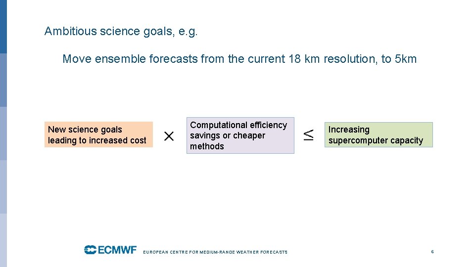
Ambitious science goals, e. g. Move ensemble forecasts from the current 18 km resolution, to 5 km New science goals leading to increased cost Computational efficiency savings or cheaper methods EUROPEAN CENTRE FOR MEDIUM-RANGE WEATHER FORECASTS Increasing supercomputer capacity 6

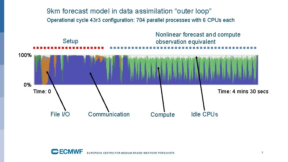
9 km forecast model in data assimilation “outer loop” Operational cycle 43 r 3 configuration: 704 parallel processes with 6 CPUs each Nonlinear forecast and compute observation equivalent Setup 100% 0% Time: 0 File I/O Time: 4 mins 30 secs Communication Compute EUROPEAN CENTRE FOR MEDIUM-RANGE WEATHER FORECASTS Idle CPUs 7

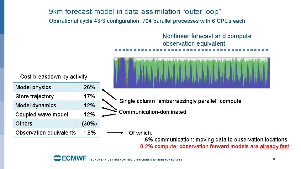
9 km forecast model in data assimilation “outer loop” Operational cycle 43 r 3 configuration: 704 parallel processes with 6 CPUs each Nonlinear forecast and compute observation equivalent Cost breakdown by activity Model physics 26% Store trajectory 17% Model dynamics 12% Coupled wave model 12% Others (30%) Observation equivalents 1. 8% Single column “embarrassingly parallel” compute Communication-dominated Of which: 1. 6% communication: moving data to observation locations 0. 2% compute: observation forward models are already fast EUROPEAN CENTRE FOR MEDIUM-RANGE WEATHER FORECASTS 8

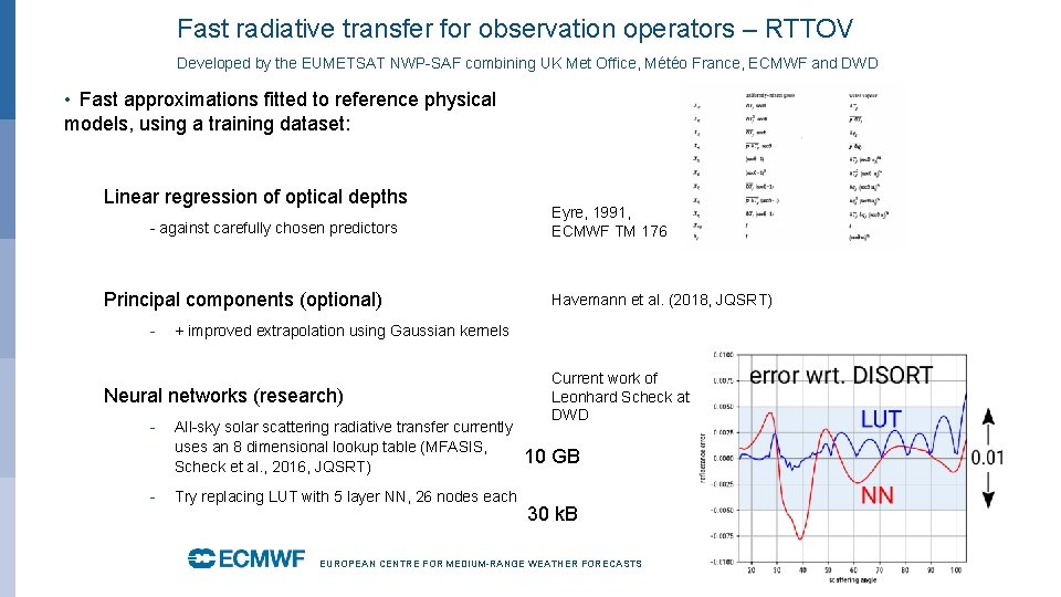
Fast radiative transfer for observation operators – RTTOV Developed by the EUMETSAT NWP-SAF combining UK Met Office, Météo France, ECMWF and DWD • Fast approximations fitted to reference physical models, using a training dataset: Linear regression of optical depths - against carefully chosen predictors Principal components (optional) - - Havemann et al. (2018, JQSRT) + improved extrapolation using Gaussian kernels Neural networks (research) - Eyre, 1991, ECMWF TM 176 All-sky solar scattering radiative transfer currently uses an 8 dimensional lookup table (MFASIS, Scheck et al. , 2016, JQSRT) Try replacing LUT with 5 layer NN, 26 nodes each Current work of Leonhard Scheck at DWD 10 GB 30 k. B EUROPEAN CENTRE FOR MEDIUM-RANGE WEATHER FORECASTS 9

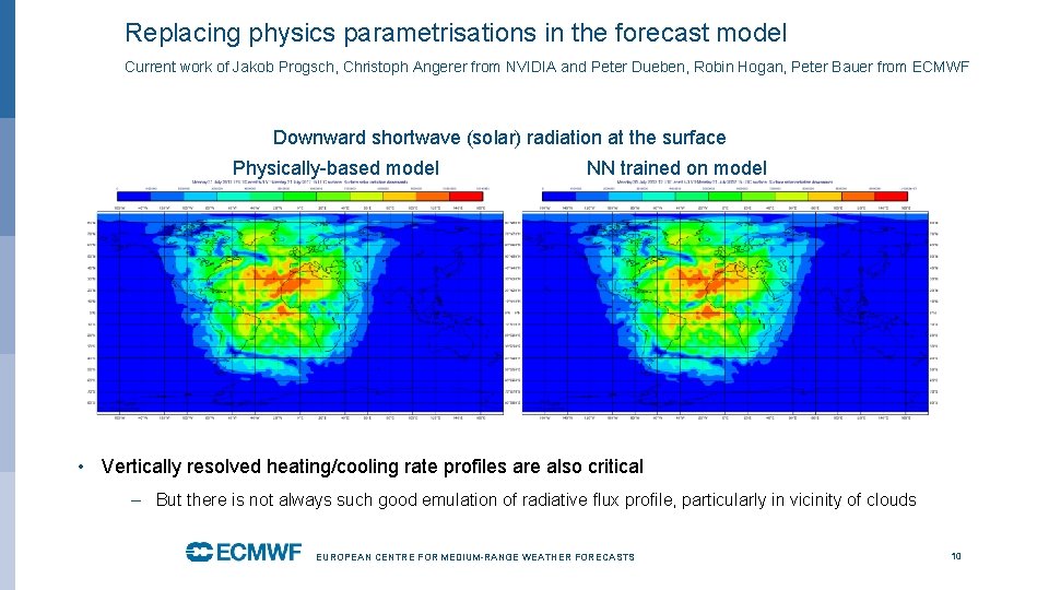
Replacing physics parametrisations in the forecast model Current work of Jakob Progsch, Christoph Angerer from NVIDIA and Peter Dueben, Robin Hogan, Peter Bauer from ECMWF Downward shortwave (solar) radiation at the surface Physically-based model NN trained on model • Vertically resolved heating/cooling rate profiles are also critical – But there is not always such good emulation of radiative flux profile, particularly in vicinity of clouds EUROPEAN CENTRE FOR MEDIUM-RANGE WEATHER FORECASTS 10

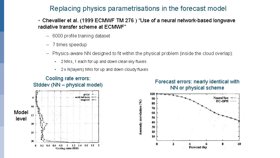
Replacing physics parametrisations in the forecast model • Chevallier et al. (1999 ECMWF TM 276 ) “Use of a neural network-based longwave radiative transfer scheme at ECMWF” – 6000 profile training dataset – 7 times speedup – Physics-aware NN designed to fit within the physical problem (inside the cloud overlap): • 2 NNs, 1 each for up and down clear-sky fluxes • 2 x N(layers) NNs for up and down cloudy fluxes Cooling rate errors: Stddev (NN – physical model) Forecast errors: nearly identical with NN or physical scheme Model level EUROPEAN CENTRE FOR MEDIUM-RANGE WEATHER FORECASTS 11

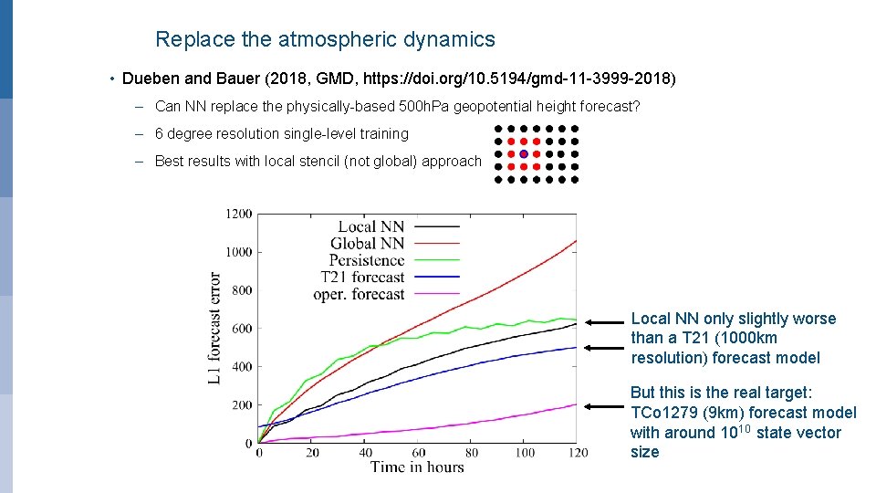
Replace the atmospheric dynamics • Dueben and Bauer (2018, GMD, https: //doi. org/10. 5194/gmd-11 -3999 -2018) – Can NN replace the physically-based 500 h. Pa geopotential height forecast? – 6 degree resolution single-level training – Best results with local stencil (not global) approach Local NN only slightly worse than a T 21 (1000 km resolution) forecast model EUROPEAN CENTRE FOR MEDIUM-RANGE WEATHER FORECASTS But this is the real target: TCo 1279 (9 km) forecast model with around 1010 state vector size 12

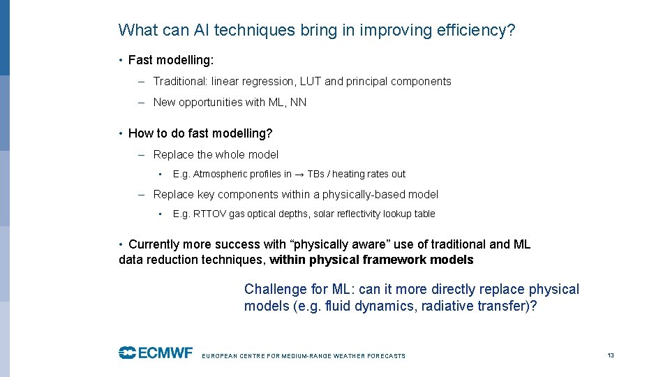
What can AI techniques bring in improving efficiency? • Fast modelling: – Traditional: linear regression, LUT and principal components – New opportunities with ML, NN • How to do fast modelling? – Replace the whole model • E. g. Atmospheric profiles in → TBs / heating rates out – Replace key components within a physically-based model • E. g. RTTOV gas optical depths, solar reflectivity lookup table • Currently more success with “physically aware” use of traditional and ML data reduction techniques, within physical framework models Challenge for ML: can it more directly replace physical models (e. g. fluid dynamics, radiative transfer)? EUROPEAN CENTRE FOR MEDIUM-RANGE WEATHER FORECASTS 13

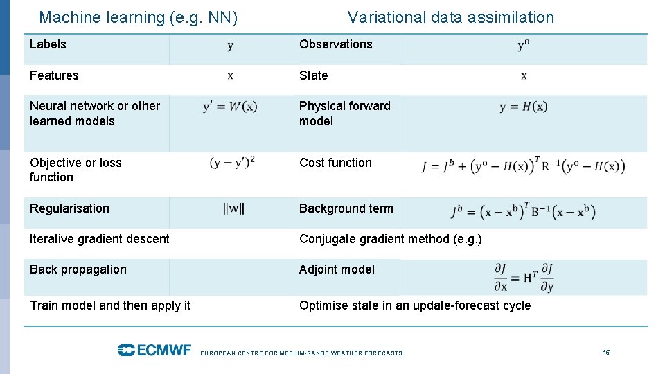
What new things can we do with AI techniques? • Replace traditional weather forecasting (NWP) entirely? • Just hang on a moment – how different are data assimilation and machine learning anyway? – AI techniques and the overlap with data assimilation have been exciting interest for years – e. g. Hsieh and Tang (1998, BAMS) – Also see Peter Jan van Leeuwen’s talk on Wednesday: “Machine learning meets data assimilation” EUROPEAN CENTRE FOR MEDIUM-RANGE WEATHER FORECASTS 14

Machine learning (e. g. NN) Variational data assimilation Labels Observations Features State Neural network or other learned models Physical forward model Objective or loss function Cost function Regularisation Background term Iterative gradient descent Conjugate gradient method (e. g. ) Back propagation Adjoint model Train model and then apply it Optimise state in an update-forecast cycle EUROPEAN CENTRE FOR MEDIUM-RANGE WEATHER FORECASTS 15

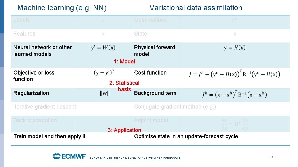
Machine learning (e. g. NN) Variational data assimilation Labels Observations Features State Neural network or other learned models Objective or loss function Regularisation Physical forward model 1: Model Cost function 2: Statistical basis Background term Iterative gradient descent Conjugate gradient method (e. g. ) Back propagation Adjoint model Train model and then apply it 3: Application Optimise state in an update-forecast cycle EUROPEAN CENTRE FOR MEDIUM-RANGE WEATHER FORECASTS 16

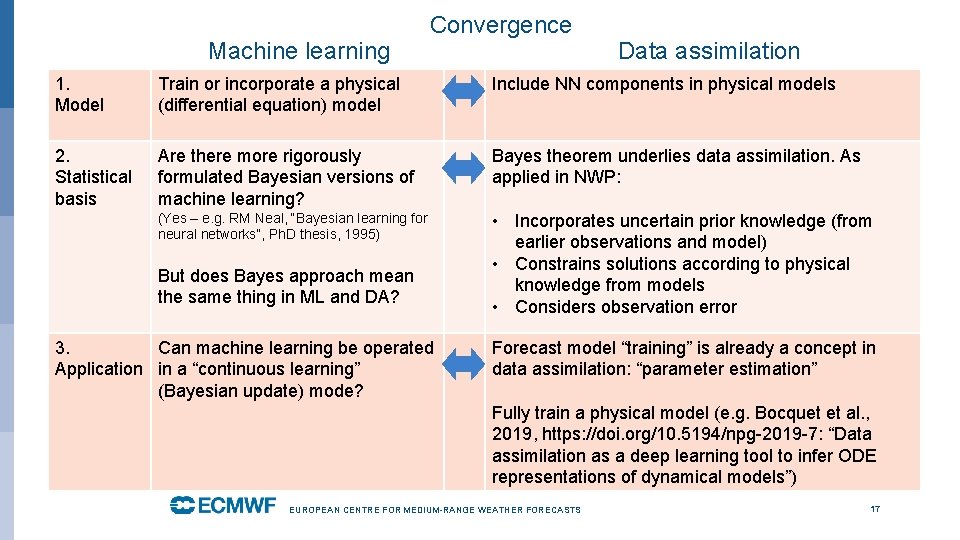
Machine learning Convergence Data assimilation 1. Model Train or incorporate a physical (differential equation) model Include NN components in physical models 2. Statistical basis Are there more rigorously formulated Bayesian versions of machine learning? Bayes theorem underlies data assimilation. As applied in NWP: (Yes – e. g. RM Neal, “Bayesian learning for neural networks”, Ph. D thesis, 1995) • Incorporates uncertain prior knowledge (from earlier observations and model) • Constrains solutions according to physical knowledge from models • Considers observation error But does Bayes approach mean the same thing in ML and DA? 3. Can machine learning be operated Application in a “continuous learning” (Bayesian update) mode? Forecast model “training” is already a concept in data assimilation: “parameter estimation” Fully train a physical model (e. g. Bocquet et al. , 2019, https: //doi. org/10. 5194/npg-2019 -7: “Data assimilation as a deep learning tool to infer ODE representations of dynamical models”) EUROPEAN CENTRE FOR MEDIUM-RANGE WEATHER FORECASTS 17

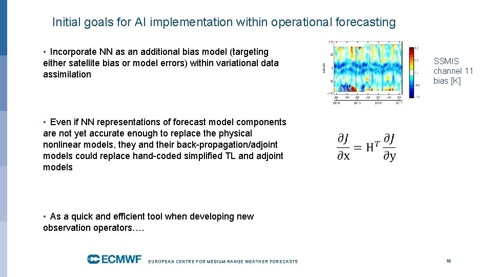
Initial goals for AI implementation within operational forecasting • Incorporate NN as an additional bias model (targeting either satellite bias or model errors) within variational data assimilation SSMIS channel 11 bias [K] • Even if NN representations of forecast model components are not yet accurate enough to replace the physical nonlinear models, they and their back-propagation/adjoint models could replace hand-coded simplified TL and adjoint models • As a quick and efficient tool when developing new observation operators…. EUROPEAN CENTRE FOR MEDIUM-RANGE WEATHER FORECASTS 18

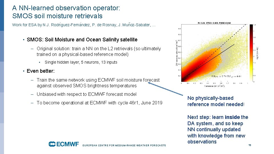
A NN-learned observation operator: SMOS soil moisture retrievals Work for ESA by N. J. Rodrı guez-Ferna ndez, P. de Rosnay, J. Mun oz-Sabater, … • SMOS: Soil Moisture and Ocean Salinity satellite – Original solution: train a NN on the L 2 retrievals (so ultimately trained on a physical-based reference model) • Single hidden layer, 5 neurons, 13 inputs • Even better: – Train the same network using ECMWF soil moisture forecast against observed SMOS brightness temperatures – Unbiased with respect to ECMWF forecast model – To become operational at ECMWF with cycle 46 r 1, June 2019 EUROPEAN CENTRE FOR MEDIUM-RANGE WEATHER FORECASTS No physically-based reference model needed! Next step: learn inside the DA system, and so keep NN continually updated with knowledge from new observations 19

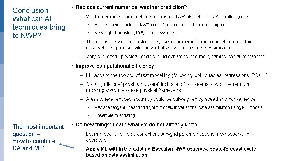
Conclusion: What can AI techniques bring to NWP? • Replace current numerical weather prediction? – Will fundamental computational issues in NWP also affect its AI challengers? • Hardest inefficiencies in NWP come from communication, not compute • Very high dimension (1010) chaotic systems – There exists a well-understood Bayesian framework for incorporating uncertain observations, prior knowledge and physical models: data assimilation – Very successful physical models (fluid dynamics, thermodynamics, radiative transfer) • Improve computational efficiency – ML adds to the toolbox of fast modelling (following lookup tables, regressions, PCs. . . ) – So far, judicious “physically aware” inclusion of ML seems to work better than throwing away the whole physical framework – Areas where reduced accuracy could be outweighed by speed and convenience: The most important question – How to combine DA and ML? • Replace tangent-linear and adjoint models in variational data assimilation using ML models • Ensemble forecasting • Do new things: Learn what we do not already know – Learn model error, bias correction, sub-grid parametrisations, new observation operators – Apply ML within the existing Bayesian NWP observe-update-forecast cycle based on data assimilation 20