Opinionated Lessons in Statistics by Bill Press 30

Opinionated Lessons in Statistics by Bill Press #30 Expectation Maximization (EM) Methods Professor William H. Press, Department of Computer Science, the University of Texas at Austin 1

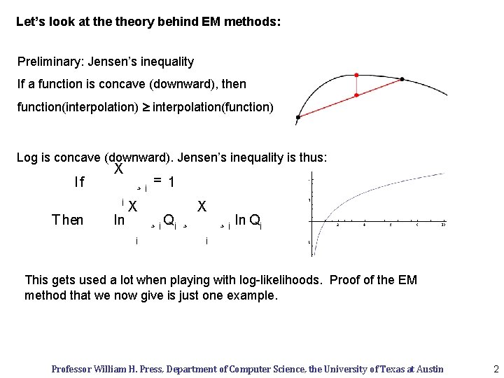
Let’s look at theory behind EM methods: Preliminary: Jensen’s inequality If a function is concave (downward), then function(interpolation) interpolation(function) Log is concave (downward). Jensen’s inequality is thus: If X i T hen ln ¸i = 1 X i ¸ i Qi ¸ X ¸ i ln Qi i This gets used a lot when playing with log-likelihoods. Proof of the EM method that we now give is just one example. Professor William H. Press, Department of Computer Science, the University of Texas at Austin 2

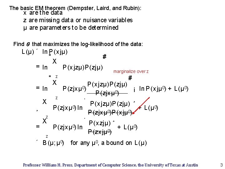
The basic EM theorem (Dempster, Laird, and Rubin): x are t he dat a z are missing dat a or nuisance variables µ are paramet ers t o be det ermined Find q that maximizes the log-likelihood of the data: L (µ) ´ ln P (x jµ) " # X = ln P (x jzµ)P (zjµ) " z X marginalize over z # P (x jzµ)P (zjµ) ¡ ln P (x jµ 0) + L (µ 0) 0 P (zjx µ ) z · ¸ X P (x jzµ)P (zjµ) 0) ¸ + P (zjx µ 0) ln L (µ P (zjx µ 0)P (x jµ 0) z · ¸ X P (xzjµ) = + L (µ 0) P (zjx µ 0) ln 0 P (zxjµ ) = ln P (zjx µ 0) z ´ B (µ; µ 0) for any µ 0, a bound on L (µ) Professor William H. Press, Department of Computer Science, the University of Texas at Austin 3

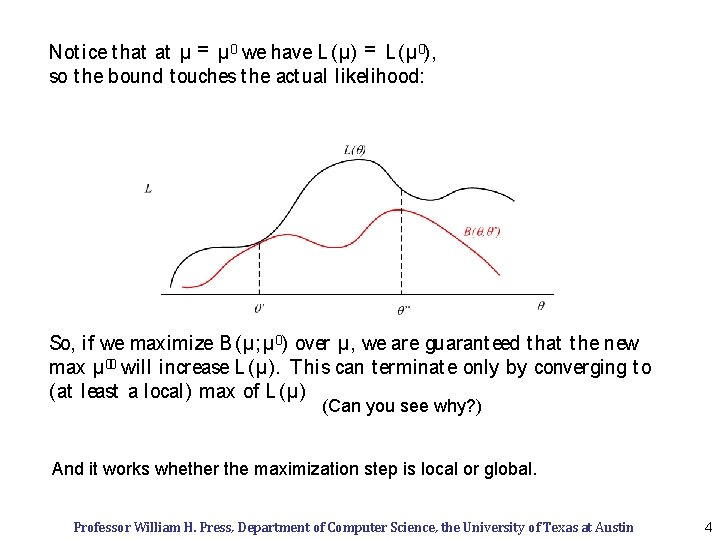
Not ice t hat at µ = µ 0 we have L (µ) = L (µ 0), so t he bound t ouches t he act ual likelihood: So, if we maximize B (µ; µ 0) over µ, we are guarant eed t hat t he new max µ 00 will increase L (µ). T his can t erminat e only by converging t o (at least a local) max of L (µ) (Can you see why? ) And it works whether the maximization step is local or global. Professor William H. Press, Department of Computer Science, the University of Texas at Austin 4

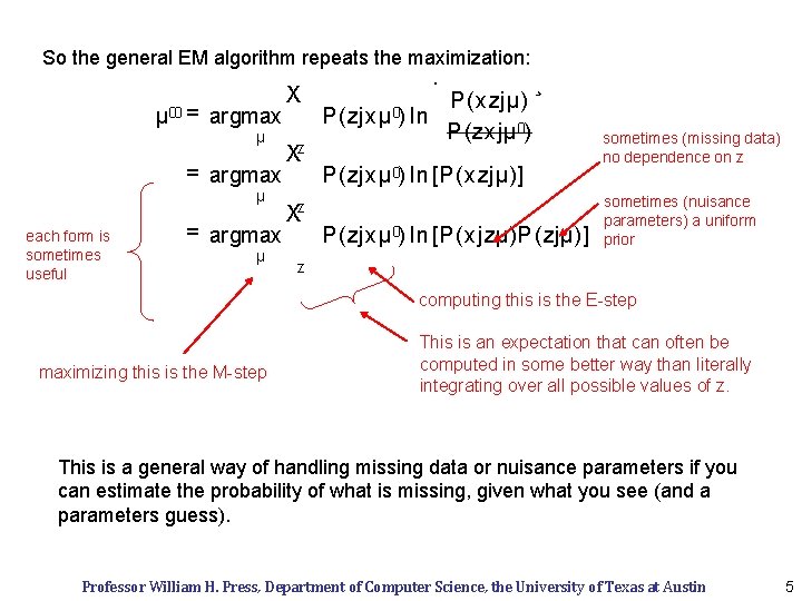
So the general EM algorithm repeats the maximization: µ 00 = argmax µ each form is sometimes useful = argmax µ X z X Xz · P (zjx µ 0) ln P (x zjµ) P (zx jµ 0) ¸ P (zjx µ 0) ln [P (xzjµ)] P (zjx µ 0) ln [P (xjzµ)P (zjµ)] sometimes (missing data) no dependence on z sometimes (nuisance parameters) a uniform prior z computing this is the E-step maximizing this is the M-step This is an expectation that can often be computed in some better way than literally integrating over all possible values of z. This is a general way of handling missing data or nuisance parameters if you can estimate the probability of what is missing, given what you see (and a parameters guess). Professor William H. Press, Department of Computer Science, the University of Texas at Austin 5

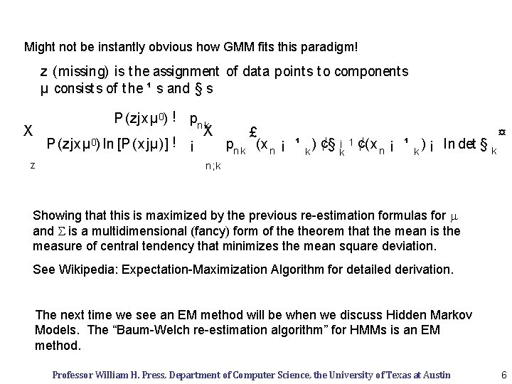
Might not be instantly obvious how GMM fits this paradigm! z (missing) is t he assignment of dat a point s t o component s µ consist s of t he ¹ s and § s P (zjxµ 0) ! pn k X X £ ¤ 0 ¡ 1 ! ¡ P (zjx µ ) ln [P (x jµ)] pn k (x n ¡ ¹ k ) ¢§ k ¢(x n ¡ ¹ k ) ¡ ln det § k z n ; k Showing that this is maximized by the previous re-estimation formulas for m and S is a multidimensional (fancy) form of theorem that the mean is the measure of central tendency that minimizes the mean square deviation. See Wikipedia: Expectation-Maximization Algorithm for detailed derivation. The next time we see an EM method will be when we discuss Hidden Markov Models. The “Baum-Welch re-estimation algorithm” for HMMs is an EM method. Professor William H. Press, Department of Computer Science, the University of Texas at Austin 6