Operator Placement for InNetwork Stream Query Processing U

Operator Placement for In-Network Stream Query Processing U. Srivastava, K. Mungala, and J. Widom, PODS 2005 ICS 280 class presentation by Iosif Lazaridis (Winter 2005)

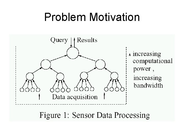
Problem Motivation

Previous Solutions • Push all data to the server: queries are processed there – Does not utilize in-network resources • Push simple filters to the leaf nodes – e. g. , “select all values >3” • Perform aggregation in intermediate nodes • But what about expensive operations? – e. g. , filters over image data, or operations involving remote lookups

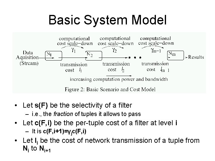
Basic System Model • Let s(F) be the selectivity of a filter – i. e. , the fraction of tuples it allows to pass • Let c(F, i) be the per-tuple cost of a filter at level i – It is c(F, i+1)=γjc(F, i) • Let li be the cost of network transmission of a tuple from Ni to Ni+1

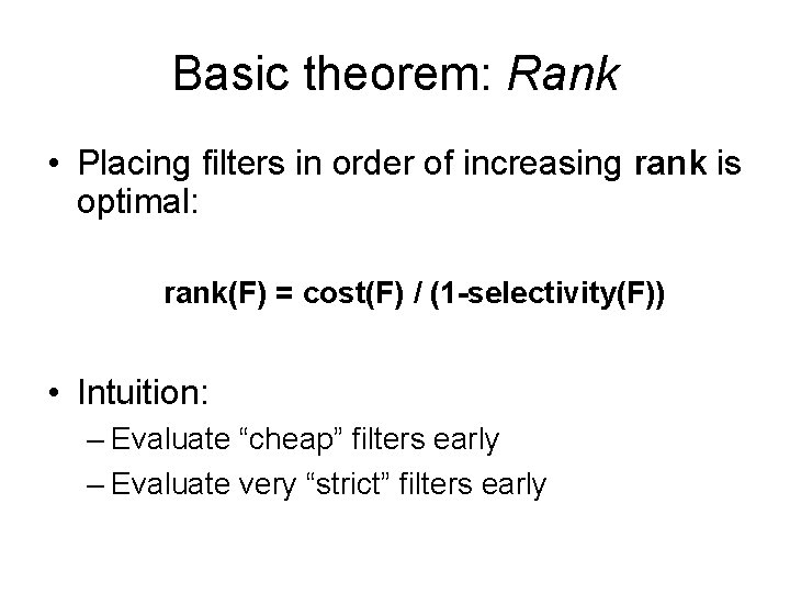
Basic theorem: Rank • Placing filters in order of increasing rank is optimal: rank(F) = cost(F) / (1 -selectivity(F)) • Intuition: – Evaluate “cheap” filters early – Evaluate very “strict” filters early

Greedy Algorithm • Let c(P, i) be the cost of plan P incurred at node i – i. e. , the cost of applying the filter and transmitting the results to i+1 – Greedy Algorithm: minimize c(P, 1) by choosing a set of filters F 1 from total set F then minimize c(P, 2) by choosing F 2 from F-F 1 etc. – Choose all filters with rank less than l 1

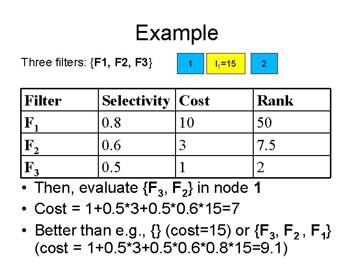
Example Three filters: {F 1, F 2, F 3} 1 l 1=15 2 Filter Selectivity Cost Rank F 1 0. 8 10 50 F 2 0. 6 3 7. 5 F 3 0. 5 1 2 • Then, evaluate {F 3, F 2} in node 1 • Cost = 1+0. 5*3+0. 5*0. 6*15=7 • Better than e. g. , {} (cost=15) or {F 3, F 2 , F 1} (cost = 1+0. 5*3+0. 5*0. 6*0. 8*15=9. 1)

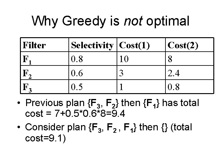
Why Greedy is not optimal Filter F 1 F 2 F 3 Selectivity 0. 8 0. 6 0. 5 Cost(1) 10 3 1 Cost(2) 8 2. 4 0. 8 • Previous plan {F 3, F 2} then {F 1} has total cost = 7+0. 5*0. 6*8=9. 4 • Consider plan {F 3, F 2 , F 1} then {} (total cost=9. 1)

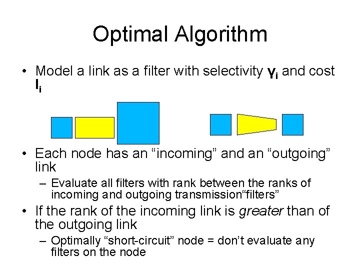
Optimal Algorithm • Model a link as a filter with selectivity γi and cost li • Each node has an “incoming” and an “outgoing” link – Evaluate all filters with rank between the ranks of incoming and outgoing transmission“filters” • If the rank of the incoming link is greater than of the outgoing link – Optimally “short-circuit” node = don’t evaluate any filters on the node

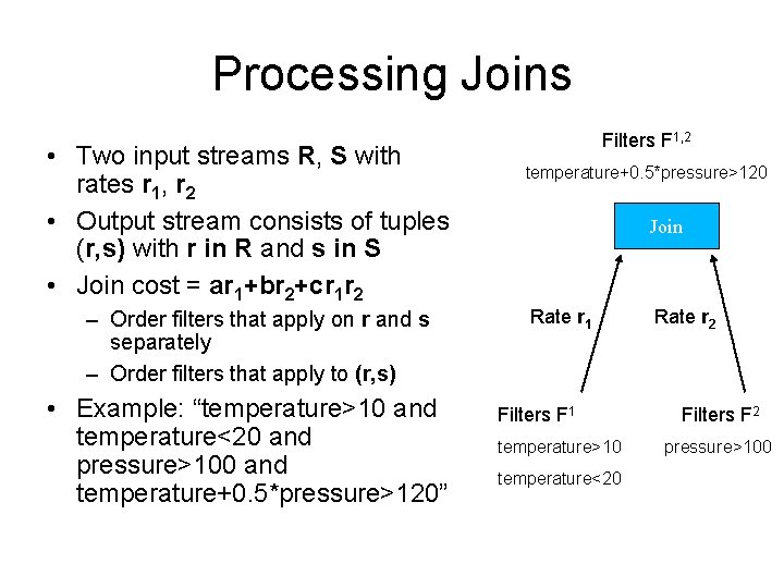
Processing Joins • Two input streams R, S with rates r 1, r 2 • Output stream consists of tuples (r, s) with r in R and s in S • Join cost = ar 1+br 2+cr 1 r 2 – Order filters that apply on r and s separately – Order filters that apply to (r, s) • Example: “temperature>10 and temperature<20 and pressure>100 and temperature+0. 5*pressure>120” Filters F 1, 2 temperature+0. 5*pressure>120 Join Rate r 1 Filters F 1 temperature>10 temperature<20 Rate r 2 Filters F 2 pressure>100

Conclusions • Systematic way to push filters into the network, taking into account their relative cost and the capabilities of nodes • Perhaps does not take into account practical issues such as broadcast communication or faults • Interesting to see practical values for γ, c, s in a real deployment.