Operations Management I Departamento de Organizacin de Empresas

Operations Management I Departamento de Organización de Empresas y Marketing Área de Organización de Empresas Dirección de Operaciones I- English teaching SECTION 2 STRATEGIC DESIGN 3º GADI- 5º DG-ADI-DER 2013 -2014 Slide presentation Chapter 7

CHAPTER 7 FACILITY LOCATION 7. 1. 7. 2. 7. 3. 7. 4. The Strategic Importance of Location Factors that Affect Location Decisions Methods of Evaluating Location Alternatives Service Location Strategy 2

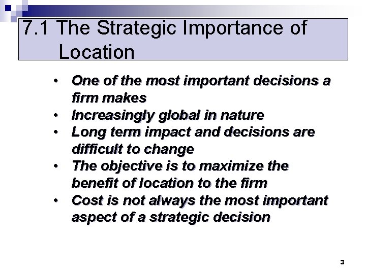
7. 1 The Strategic Importance of Location • One of the most important decisions a firm makes • Increasingly global in nature • Long term impact and decisions are difficult to change • The objective is to maximize the benefit of location to the firm • Cost is not always the most important aspect of a strategic decision 3

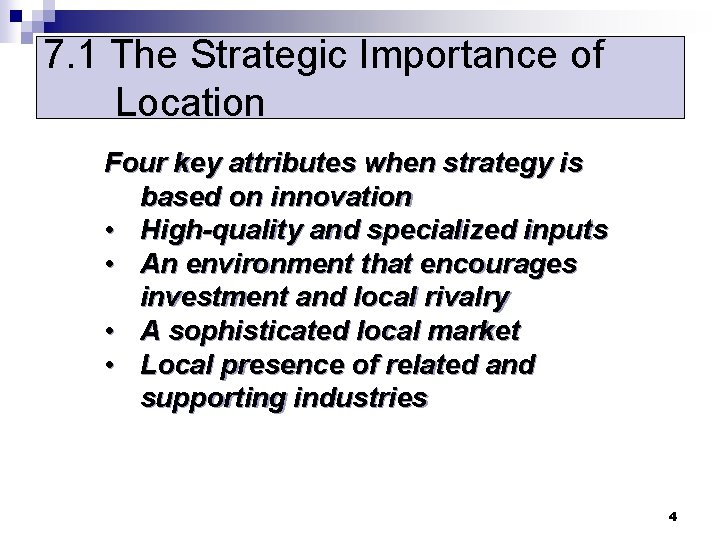
7. 1 The Strategic Importance of Location Four key attributes when strategy is based on innovation • High-quality and specialized inputs • An environment that encourages investment and local rivalry • A sophisticated local market • Local presence of related and supporting industries 4

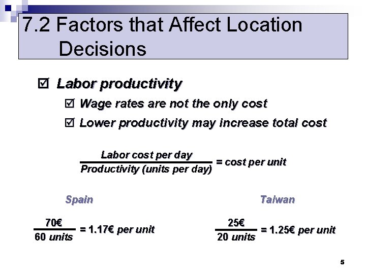
7. 2 Factors that Affect Location Decisions þ Labor productivity þ Wage rates are not the only cost þ Lower productivity may increase total cost Labor cost per day = cost per unit Productivity (units per day) Spain 70€ = 1. 17€ per unit 60 units Taiwan 25€ = 1. 25€ per unit 20 units 5

7. 2 Factors that Affect Location Decisions þ Exchange rates and currency risks þ Can have a significant impact on cost structure þ Rates change over time þ Costs þ Tangible - easily measured costs such as utilities, labor, materials, taxes þ Intangible - less easy to quantify and include education, public transportation, community, quality-of-life 6

7. 2 Factors that Affect Location Decisions þ Attitudes þ National, state, local governments toward private and intellectual property, zoning, pollution, employment stability þ Worker attitudes towards turnover, unions, absenteeism þ Globally cultures have different attitudes towards punctuality, legal, and ethical issues 7

7. 2 Factors that Affect Location Decisions þ Proximity to markets þ Very important to services þ JIT systems or high transportation costs may make it important to manufacturers þ Proximity to suppliers þ Perishable goods, high transportation costs, bulky products 8

7. 2 Factors that Affect Location Decisions þ Proximity to competitors þ Called clustering þ Often driven by resources such as natural, information, capital, talent þ Found in both manufacturing and service industries 9

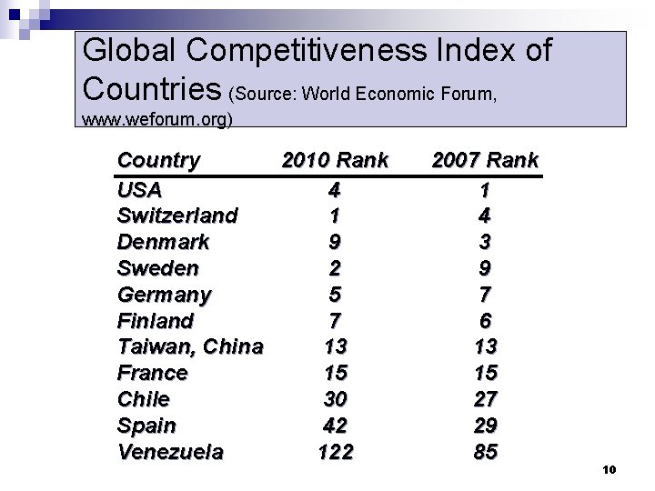
Global Competitiveness Index of Countries (Source: World Economic Forum, www. weforum. org) Country 2010 Rank USA 4 Switzerland 1 Denmark 9 Sweden 2 Germany 5 Finland 7 Taiwan, China 13 France 15 Chile 30 Spain 42 Venezuela 122 2007 Rank 1 4 3 9 7 6 13 15 27 29 85 10

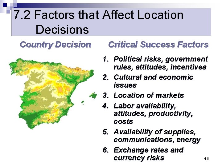
7. 2 Factors that Affect Location Decisions Country Decision Critical Success Factors 1. Political risks, government rules, attitudes, incentives 2. Cultural and economic issues 3. Location of markets 4. Labor availability, attitudes, productivity, costs 5. Availability of supplies, communications, energy 6. Exchange rates and 11 currency risks

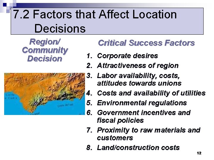
7. 2 Factors that Affect Location Decisions Region/ Community Decision Critical Success Factors 1. Corporate desires 2. Attractiveness of region 3. Labor availability, costs, attitudes towards unions 4. Costs and availability of utilities 5. Environmental regulations 6. Government incentives and fiscal policies 7. Proximity to raw materials and customers 8. Land/construction costs 12

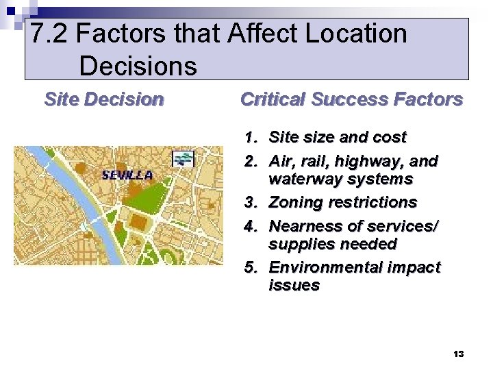
7. 2 Factors that Affect Location Decisions Site Decision Critical Success Factors 1. Site size and cost 2. Air, rail, highway, and waterway systems 3. Zoning restrictions 4. Nearness of services/ supplies needed 5. Environmental impact issues 13

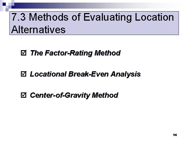
7. 3 Methods of Evaluating Location Alternatives þ The Factor-Rating Method þ Locational Break-Even Analysis þ Center-of-Gravity Method 14

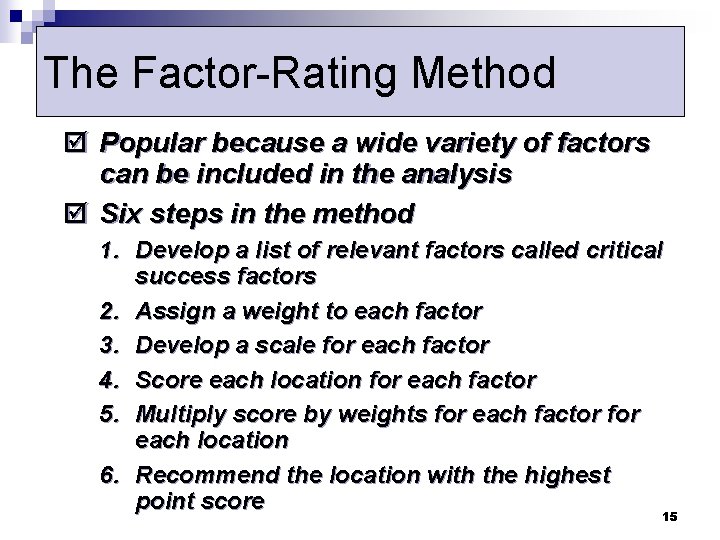
The Factor-Rating Method þ Popular because a wide variety of factors can be included in the analysis þ Six steps in the method 1. Develop a list of relevant factors called critical success factors 2. Assign a weight to each factor 3. Develop a scale for each factor 4. Score each location for each factor 5. Multiply score by weights for each factor for each location 6. Recommend the location with the highest point score 15

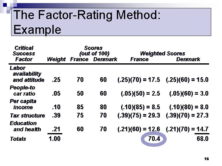
The Factor-Rating Method: Example Critical Success Factor Labor availability and attitude People-to car ratio Per capita income Tax structure Education and health Totals Scores (out of 100) Weight France Denmark Weighted Scores France Denmark . 25 70 60 . 05 50 60 . 10. 39 85 75 80 70 (. 10)(85) = 8. 5 (. 10)(80) = 8. 0 (. 39)(75) = 29. 3 (. 39)(70) = 27. 3 . 21 60 70 (. 21)(60) = 12. 6 (. 21)(70) = 14. 7 1. 00 (. 25)(70) = 17. 5 (. 25)(60) = 15. 0 (. 05)(50) = 2. 5 70. 4 (. 05)(60) = 3. 0 68. 0 16

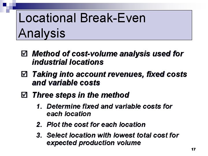
Locational Break-Even Analysis þ Method of cost-volume analysis used for industrial locations þ Taking into account revenues, fixed costs and variable costs þ Three steps in the method 1. Determine fixed and variable costs for each location 2. Plot the cost for each location 3. Select location with lowest total cost for expected production volume 17

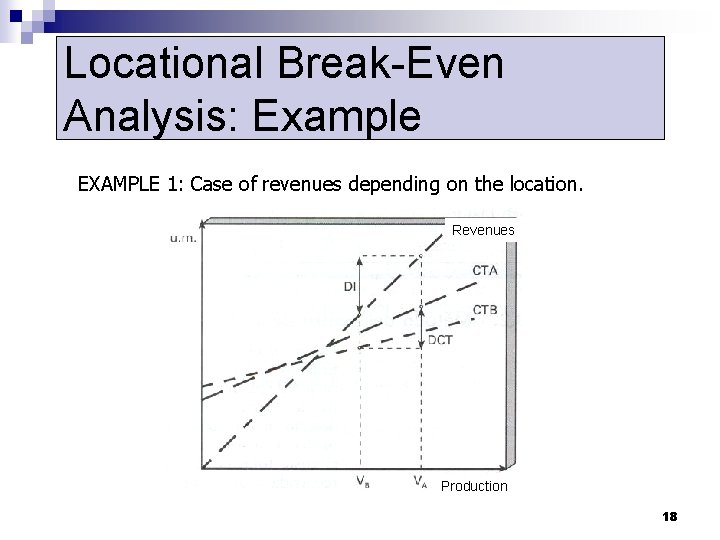
Locational Break-Even Analysis: Example EXAMPLE 1: Case of revenues depending on the location. Revenues Production 18

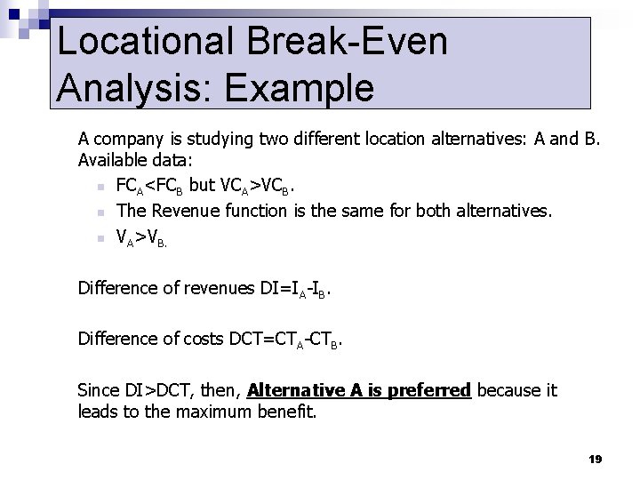
Locational Break-Even Analysis: Example A company is studying two different location alternatives: A and B. Available data: n FCA<FCB but VCA>VCB. n The Revenue function is the same for both alternatives. n VA>VB. Difference of revenues DI=IA-IB. Difference of costs DCT=CTA-CTB. Since DI>DCT, then, Alternative A is preferred because it leads to the maximum benefit. 19

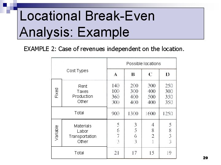
Locational Break-Even Analysis: Example EXAMPLE 2: Case of revenues independent on the location. Possible locations Fixed Cost Types Rent Taxes Production Other Variable Total Materials Labor Transportation Other Total 20

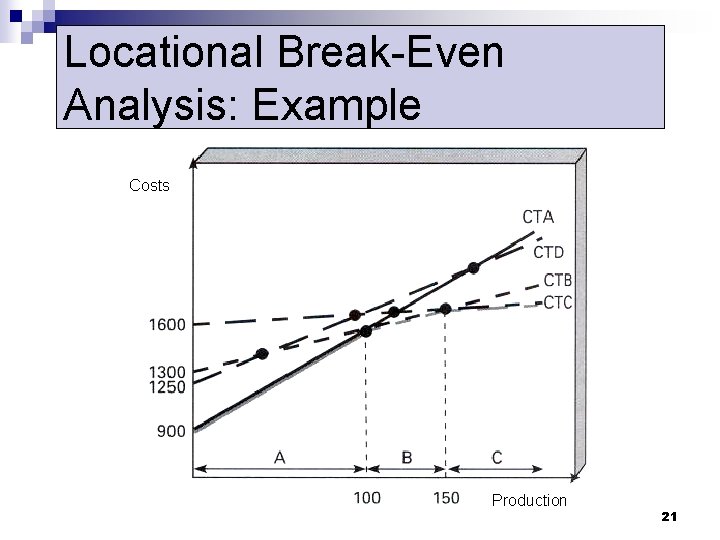
Locational Break-Even Analysis: Example Costs Production 21

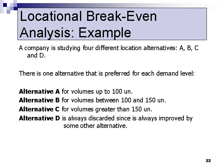
Locational Break-Even Analysis: Example A company is studying four different location alternatives: A, B, C and D. There is one alternative that is preferred for each demand level: Alternative A for volumes up to 100 un. Alternative B for volumes between 100 and 150 un. Alternative C for volumes greater than 150 un. Alternative D is always discarded since is always improved by some other alternative. 22

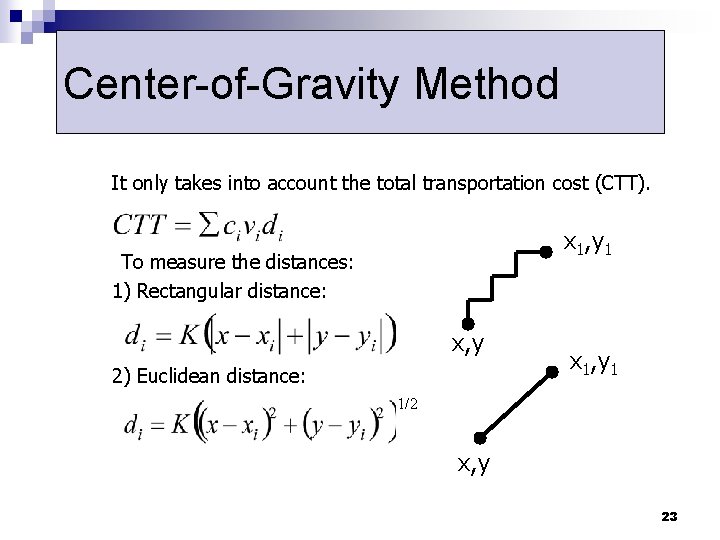
Center-of-Gravity Method It only takes into account the total transportation cost (CTT). x 1, y 1 To measure the distances: 1) Rectangular distance: x, y 2) Euclidean distance: x 1, y 1 1/2 x, y 23

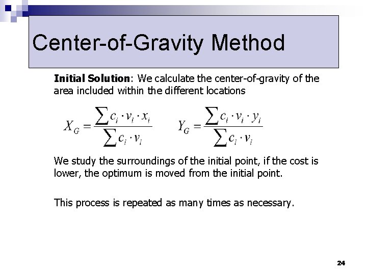
Center-of-Gravity Method Initial Solution: We calculate the center-of-gravity of the area included within the different locations We study the surroundings of the initial point, if the cost is lower, the optimum is moved from the initial point. This process is repeated as many times as necessary. 24

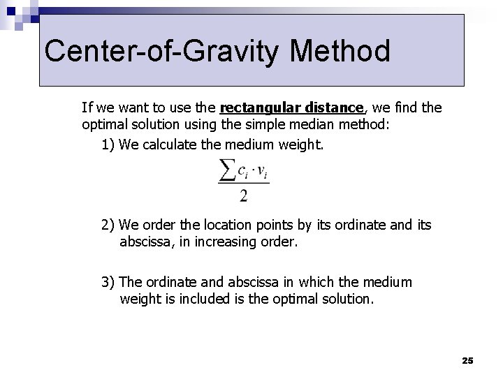
Center-of-Gravity Method If we want to use the rectangular distance, we find the optimal solution using the simple median method: 1) We calculate the medium weight. 2) We order the location points by its ordinate and its abscissa, in increasing order. 3) The ordinate and abscissa in which the medium weight is included is the optimal solution. 25

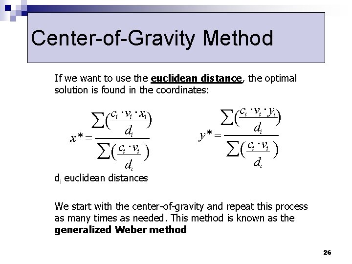
Center-of-Gravity Method If we want to use the euclidean distance, the optimal solution is found in the coordinates: ci × vi × xi å( d ) i x* = c i × vi å( ) di ci × vi × yi å( d ) i y* = å( ci × vi ) di di euclidean distances We start with the center-of-gravity and repeat this process as many times as needed. This method is known as the generalized Weber method 26

EXAMPLE 1: We are searching for a new plant location so that transportation costs are minimized for raw materials from the source (Fi) to the new plant, and for finished products from the new plant to the destination points (Mj). In the following table we show the coordinates for each of the points, the unit transportation costs (ci) and the average quantity transported by month (vi). Points Coordinates 27

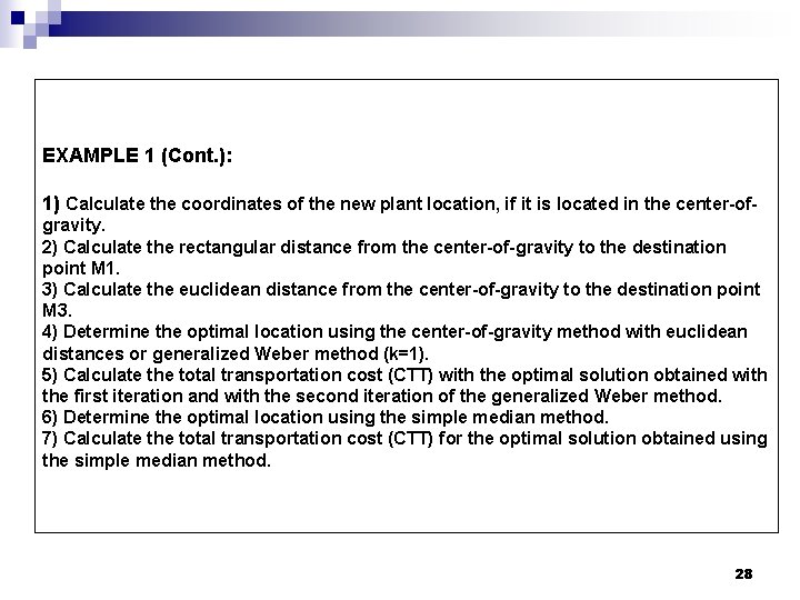
EXAMPLE 1 (Cont. ): 1) Calculate the coordinates of the new plant location, if it is located in the center-ofgravity. 2) Calculate the rectangular distance from the center-of-gravity to the destination point M 1. 3) Calculate the euclidean distance from the center-of-gravity to the destination point M 3. 4) Determine the optimal location using the center-of-gravity method with euclidean distances or generalized Weber method (k=1). 5) Calculate the total transportation cost (CTT) with the optimal solution obtained with the first iteration and with the second iteration of the generalized Weber method. 6) Determine the optimal location using the simple median method. 7) Calculate the total transportation cost (CTT) for the optimal solution obtained using the simple median method. 28

Determine the following: Calculate the coordinates of the new plant location, if it is located in the center-ofgravity. Points Coordinates Calculate the rectangular distance from the center-of-gravity to the destination point M 1: Calculate the euclidean distance from the center-of-gravity to the destination point M 3: 29

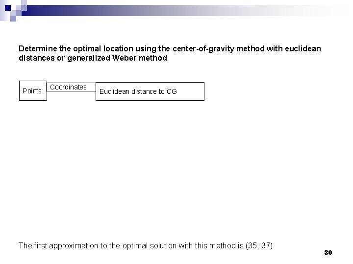
Determine the optimal location using the center-of-gravity method with euclidean distances or generalized Weber method Points Coordinates Euclidean distance to CG The first approximation to the optimal solution with this method is (35, 37) 30

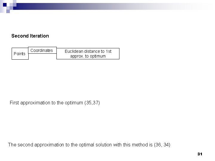
Second Iteration Points Coordinates Euclidean distance to 1 st approx. to optimum First approximation to the optimum (35, 37) The second approximation to the optimal solution with this method is (36, 34) 31

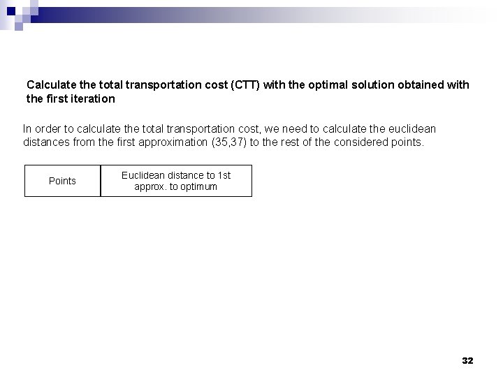
Calculate the total transportation cost (CTT) with the optimal solution obtained with the first iteration In order to calculate the total transportation cost, we need to calculate the euclidean distances from the first approximation (35, 37) to the rest of the considered points. Points Euclidean distance to 1 st approx. to optimum 32

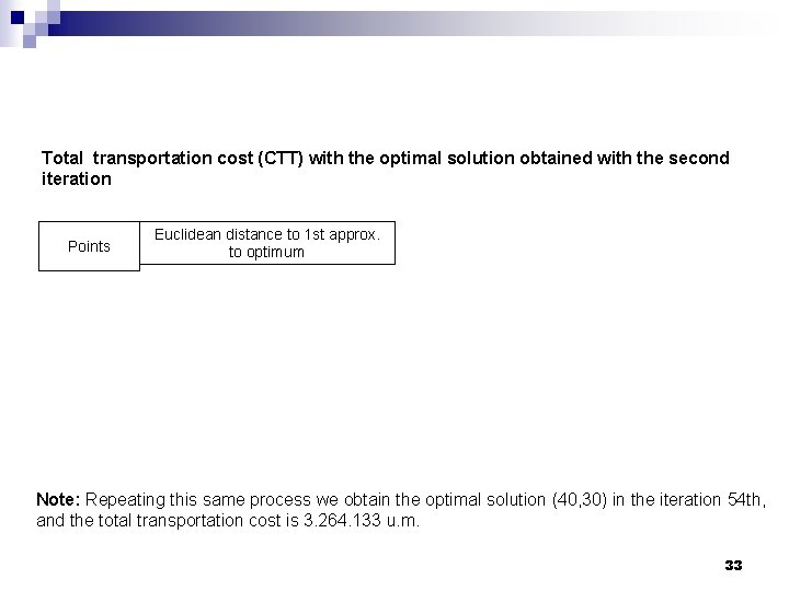
Total transportation cost (CTT) with the optimal solution obtained with the second iteration Points Euclidean distance to 1 st approx. to optimum Note: Repeating this same process we obtain the optimal solution (40, 30) in the iteration 54 th, and the total transportation cost is 3. 264. 133 u. m. 33

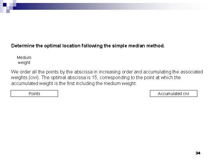
Determine the optimal location following the simple median method. Medium weight We order all the points by the abscissa in increasing order and accumulating the associated weights (civi). The optimal abscissa is 15, corresponding to the point at which the accumulated weight is the first including the medium weight. Points Accumulated civi 34

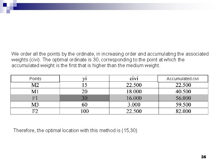
We order all the points by the ordinate, in increasing order and accumulating the associated weights (civi). The optimal ordinate is 30, corresponding to the point at which the accumulated weight is the first that is higher than the medium weight. Points Accumulated civi Therefore, the optimal location with this method is (15, 30) 35

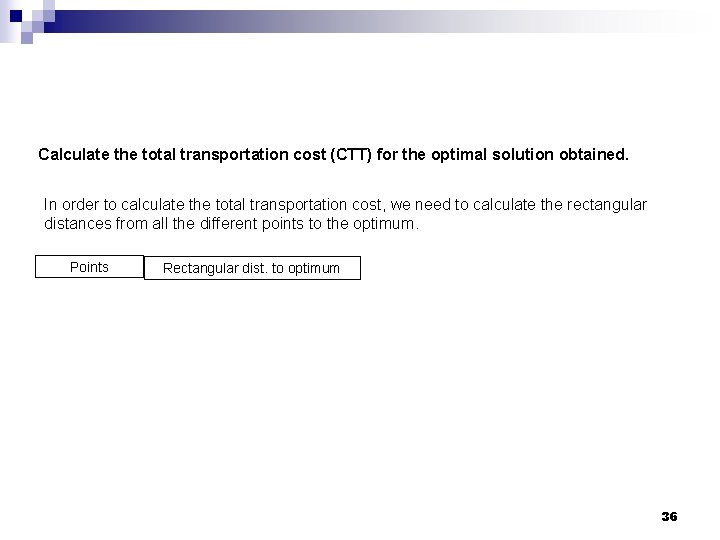
Calculate the total transportation cost (CTT) for the optimal solution obtained. In order to calculate the total transportation cost, we need to calculate the rectangular distances from all the different points to the optimum. Points Rectangular dist. to optimum 36

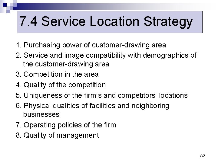
7. 4 Service Location Strategy 1. Purchasing power of customer-drawing area 2. Service and image compatibility with demographics of the customer-drawing area 3. Competition in the area 4. Quality of the competition 5. Uniqueness of the firm’s and competitors’ locations 6. Physical qualities of facilities and neighboring businesses 7. Operating policies of the firm 8. Quality of management 37