Operating Systems Virtual Memory Virtual Memory Topics 1

Operating Systems Virtual Memory

Virtual Memory Topics 1. Memory Hierarchy 2. Why Virtual Memory 3. Virtual Memory Issues 4. Virtual Memory Solutions 5. Locality of Reference 6. Virtual Memory with Segmentation 7. Page Memory Architecture

Topics (continued) 8. Algorithm for Virtual Paged Memory 9. Paging Example 10. Replacement Algorithms 11. Working Set Characteristics

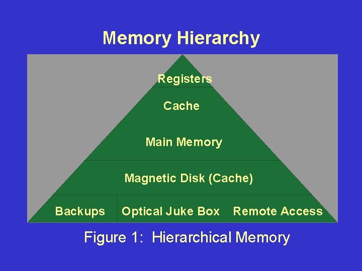
Memory Hierarchy Registers Cache Main Memory Magnetic Disk (Cache) Backups Optical Juke Box Remote Access Figure 1: Hierarchical Memory

Why Virtual Memory? Users frequently have a speed vs. cost decision. Users want: 1. To extend fast but inexpensive memory with slower but cheaper memory. 2. To have fast access.

Virtual Memory Issues 1. Fetch Strategy - Retrieval from secondary storage (a) Demand - on an as needed basis (b) Anticipatory - aka Prefetching or Prepaging 2. Placement Strategies - Where does the data go?

Virtual Memory Issues (continued) 3. Replacement Strategies - Which page or segment to load and which one gets swapped out? We seek to avoid overly frequent replacement (called thrashing).

Virtual Memory Solutions Virtual memory solutions employ: 1. Segmentation 2. Paging 3. Combined Paging and Segmentation - Current trend.

Locality of Reference Locality of reference by observing that process tend to reference storage in nonuniform, highly localized patterns. Locality can be: 1. Temporal - Looping, subroutines, stacks, counter variables. 2. Spatial - Array traversals, sequential code, data encapsulation.

Locality of Reference (continued) Things that hurt locality: 1. Frequently taken conditional branches 2. Linked data structures 3. Random Access patterns in storage

Virtual Memory with Segmentation Only Segmentation provides protection and relocation so: 1. The operating system can swap segments out not in use. 2. Data objects can be assigned their own data segments they do not fit in an existing data segment. 3. Sharing can be facilitated using the protection mechanism.

Virtual Memory with Segmentation Only (continued) 4. No internal fragmentation. 5. Main memory has external fragmentation. Pure segmented solutions are not currently in fashion. These techniques combine well with paging (as shown later)

Virtual Paged Memory Architecture • Paging is frequently used to increase the logical memory space. • Page frames (or frames for short) are the unit of placement/replacement. • A page which has been updated since it was loaded is dirty, otherwise it is clean. • A page frame may be locked in memory (not replaceable). (e. g. O/S Kernel)

Virtual Paged Memory Architecture (continued) Some architectural challenges include: 1. Protection kept for each page. 2. Dirty/clean/lock status kept for each page. 3. Instructions may span pages. 4. An instructions operands may span pages. 5. Iterative instructions (e. g Intel 80 x 86) may have data spanning many pages.

The Algorithm for Virtual Paged Memory For each reference do the following: 1. If the page is resident, use it. 2. If there is an available page, allocate it and load the required nonresident page.

The Algorithm for Virtual Paged Memory (continued) 3. If there is no available frames, then: (a) Select a page to be removed (the victim). (b) If the victim is dirty, write to secondary storage. (c) Load the nonresident page into the victim’s frame.

The Algorithm for Virtual Paged Memory (continued) Stallings [3] uses the term page fault to mean replacement operations. Many others (including your instructor) use page fault to refer to loading any pages (not just replacement).

Demand Page Replacement Let Mt be the set of resident pages at time t. For a program that runs T steps the memory state is: M 0, M 1, M 2, . . , MT Memory is usually empty when starting a process, so M 0= 0.

Demand Page Replacement (continued) Assume that real memory has m page frames, so |Mt| m. Let Xt be the set of newly loaded pages and Yt be the set of newly replaced pages at time t. Let y Mt be some page in Mt (if nonempty).

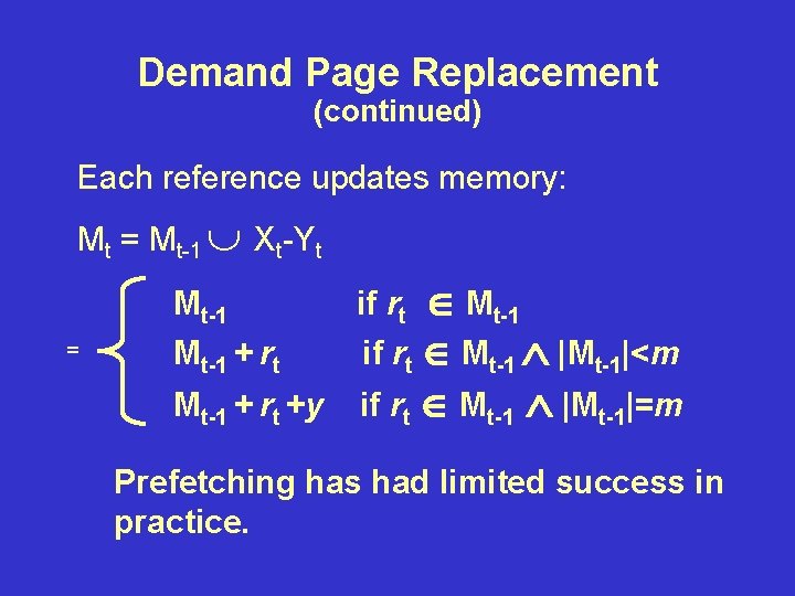
Demand Page Replacement (continued) Each reference updates memory: Mt = Mt-1 Xt-Yt = Mt-1 + rt +y if rt Mt-1 |Mt-1|<m if rt Mt-1 |Mt-1|=m Prefetching has had limited success in practice.

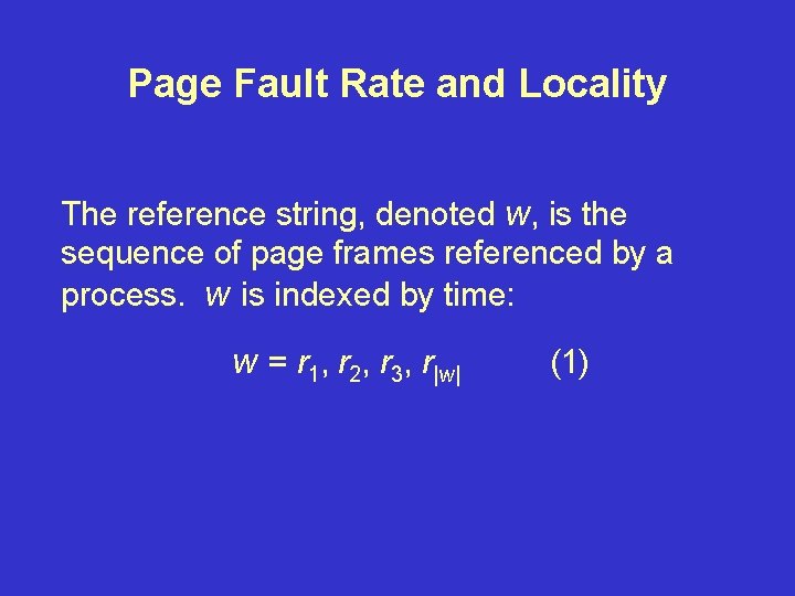
Page Fault Rate and Locality The reference string, denoted w, is the sequence of page frames referenced by a process. w is indexed by time: w = r 1 , r 2 , r 3 , r| w | (1)

Cost Measures For Paging For each level of hierarchy, a page is either: 1. is resident with the probability 1 -p and can be referenced with cost 1 2. is not resident with probability p and must be loaded with a cost F

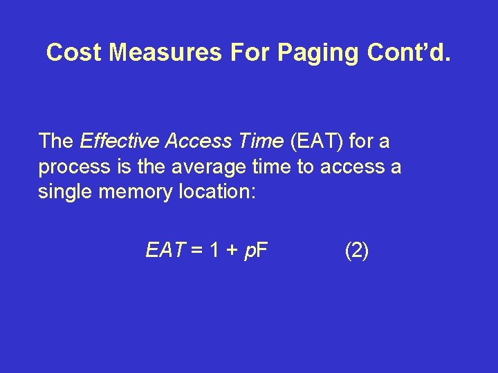
Cost Measures For Paging Cont’d. The Effective Access Time (EAT) for a process is the average time to access a single memory location: EAT = 1 + p. F (2)

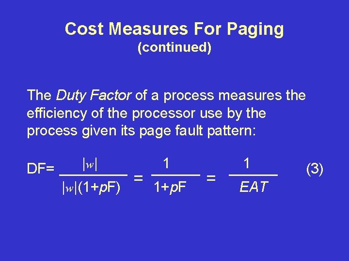
Cost Measures For Paging (continued) The Duty Factor of a process measures the efficiency of the processor use by the process given its page fault pattern: DF= | w| _______ 1 _____ = |w|(1+p. F) 1+p. F = 1 _____ EAT (3)

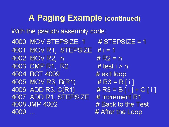
A Paging Example Consider the following example [? ] : STEPSIZE = 1; for (i = 1; i <= n; i = i + STEPSIZE) { A[ i ] = B[ i ] + C[ i ] ; }

A Paging Example (continued) With the pseudo assembly code: 4000 MOV STEPSIZE, 1 4001 MOV R 1, STEPSIZE 4002 MOV R 2, n 4003 CMP R 1, R 2 4004 BGT 4009 4005 MOV R 3, B(R 1) 4006 ADD R 3, C(R 1) 4007 ADD R 1, STEPSIZE 4008 JMP 4002 4009. . . # STEPSIZE = 1 #i=1 # R 2 = n # test i > n # exit loop # R 3 = B [ i ] + C [ i ] # Increment R 1 # Back to the Test # After the Loop

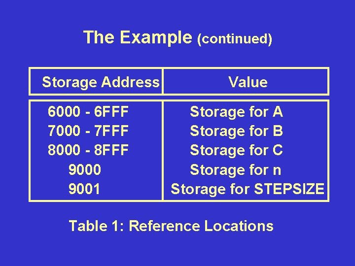
The Example (continued) Storage Address 6000 - 6 FFF 7000 - 7 FFF 8000 - 8 FFF 9000 9001 Value Storage for A Storage for B Storage for C Storage for n Storage for STEPSIZE Table 1: Reference Locations

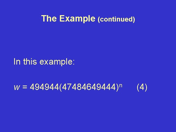
The Example (continued) In this example: w = 494944(47484649444)n (4)

Locality in Paged Memory If we have at least 5 frames of 64 KB then we know that the program does 5 page loads and no swaps. Otherwise, how many page faults are there?

Locality in Paged Memory Page Frame 10 Access Patterns in A[i]=B[i]+C[i], i=1. . 100 8 6 4 2 0 200 400 600 800 1000 1200 Time of Reference Page Trace of Example for n=100

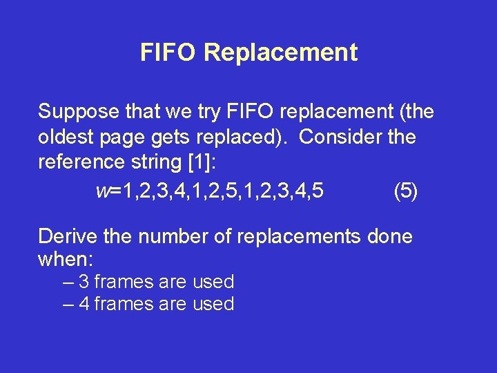
FIFO Replacement Suppose that we try FIFO replacement (the oldest page gets replaced). Consider the reference string [1]: w=1, 2, 3, 4, 1, 2, 5, 1, 2, 3, 4, 5 (5) Derive the number of replacements done when: – 3 frames are used – 4 frames are used

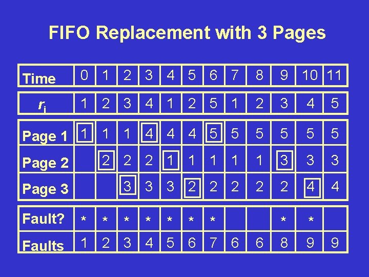
FIFO Replacement with 3 Pages Time 0 1 2 3 4 5 6 7 8 9 10 11 ri 1 2 3 4 1 2 5 1 2 3 4 5 Page 1 1 4 4 4 5 5 5 Page 2 2 1 1 1 3 3 3 Page 3 3 2 2 2 4 4 Fault? * * * * 1 2 3 4 5 6 7 6 6 * 8 * 9 9 Faults

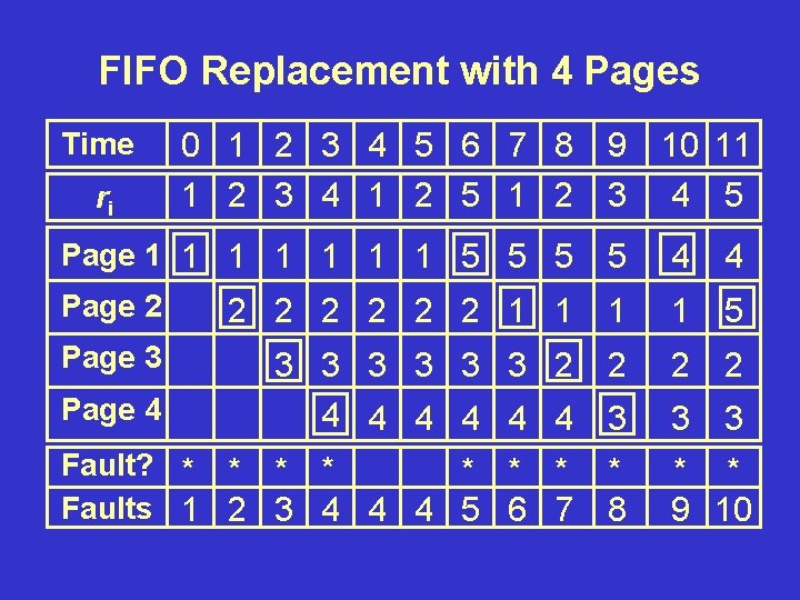
FIFO Replacement with 4 Pages Time 0 1 2 3 4 5 6 7 8 9 10 11 ri 1 2 3 4 1 2 5 1 2 3 4 5 Page 1 1 1 1 5 5 4 4 Page 2 2 2 2 1 1 5 Page 3 3 3 3 2 4 4 4 2 2 2 3 3 3 Fault? * * * * Faults 1 2 3 4 4 4 5 6 7 * 8 * * 9 10 Page 4

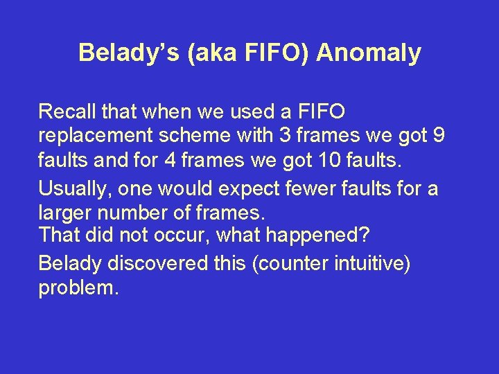
Belady’s (aka FIFO) Anomaly Recall that when we used a FIFO replacement scheme with 3 frames we got 9 faults and for 4 frames we got 10 faults. Usually, one would expect fewer faults for a larger number of frames. That did not occur, what happened? Belady discovered this (counter intuitive) problem.

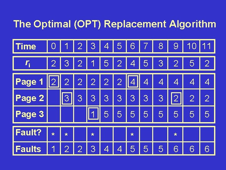
The Optimal (OPT) Replacement Algorithm The optimal (OPT) is to select the victim such that it is the page that will be reference the longest time into the future. Note that on the following table at t=9, Page 1 could have been the victim too.

The Optimal (OPT) Replacement Algorithm Time 0 1 2 3 4 5 6 7 8 9 10 11 ri 2 3 2 1 5 2 4 5 3 2 5 2 Page 1 2 2 2 4 4 4 Page 2 3 3 3 3 2 2 2 Page 3 1 5 5 5 5 Fault? * * 1 2 2 3 4 4 5 5 5 * 6 6 6 Faults

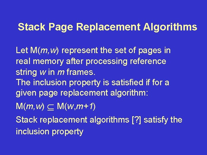
Stack Page Replacement Algorithms Let M(m, w) represent the set of pages in real memory after processing reference string w in m frames. The inclusion property is satisfied if for a given page replacement algorithm: M(m, w) M(w, m+1) Stack replacement algorithms [? ] satisfy the inclusion property

Stack Page Replacement Algorithms (continued) e. g. FIFO is NOT a stack page replacement algorithm (inclusion is NOT satisfied), while OPT is.

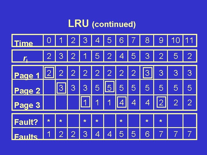
Least Recently Used (LRU) LRU is a popular stack page replacement strategy. Pages are ordered by time of last access, with the page used furthest into the past being removed.

LRU (continued) Time 0 1 2 3 4 5 6 7 8 9 10 11 ri 2 3 2 1 5 2 4 5 3 2 5 2 Page 1 2 2 2 2 3 3 Page 2 3 3 3 5 5 5 5 Page 3 1 1 1 4 4 4 2 2 2 Fault? * * * 1 2 2 3 4 4 5 5 * 6 * 7 7 7 Faults

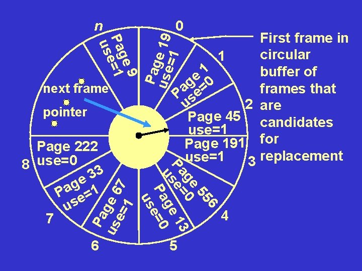
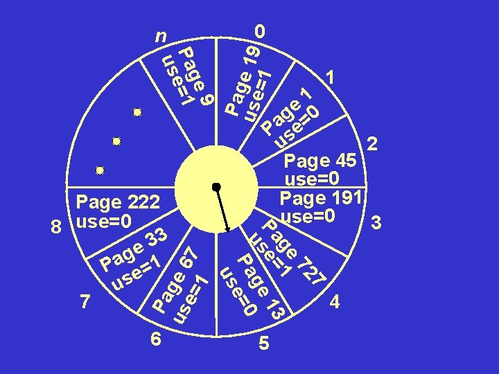
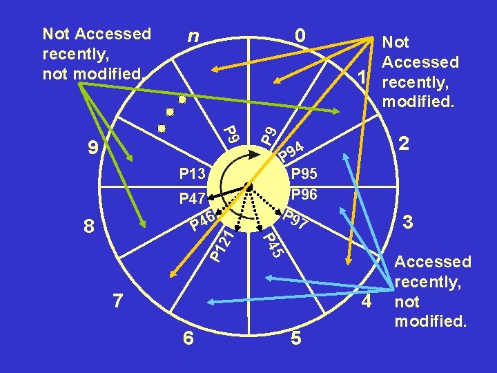
Clock Replacement Algorithms Clock replacement algorithms are stack algorithms. The simplest style marks pages with use=1 when referenced and use=0 upon a circular scan.

0 e 9 Pag =1 use next frame pointer Pa us ge 6 e= 7 1 6 6 55 ge 0 13 Pa e= us ge Pa e=0 us Page 222 8 use=0 3 3 e g 1 a P e= us 7 First frame in circular 1 1 buffer of e g =0 a frames that P se 2 are u Page 45 candidates use=1 Page 191 for use=1 3 replacement Pag use e 19 =1 n 5 4

Simple Clock Replacement The first page encountered with use=0 is selected. The final position of the previous scan is used to start the next scan.

e 9 Pag =1 use Pa us ge 6 e= 7 1 6 1 1 e 0 g Pa se= 2 u Page 45 use=0 Page 191 use=0 3 7 72 ge 1 13 Pa e= us ge Pa e=0 us Page 222 8 use=0 3 3 e g 1 a P e= us 7 Pag use e 19 =1 0 n 5 4

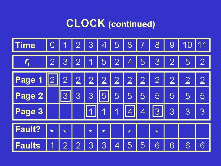
Simple Clock (CLOCK) CLOCK is a popular stack page replacement strategy, pages in use are underlined.

CLOCK (continued) Time 0 1 2 3 4 5 6 7 8 9 10 11 ri 2 3 2 1 5 2 4 5 3 2 5 2 Page 1 2 2 2 Page 2 3 3 3 5 5 5 5 Page 3 1 1 1 4 4 3 3 Fault? * * * 1 2 2 3 3 4 5 5 * 6 6 Faults

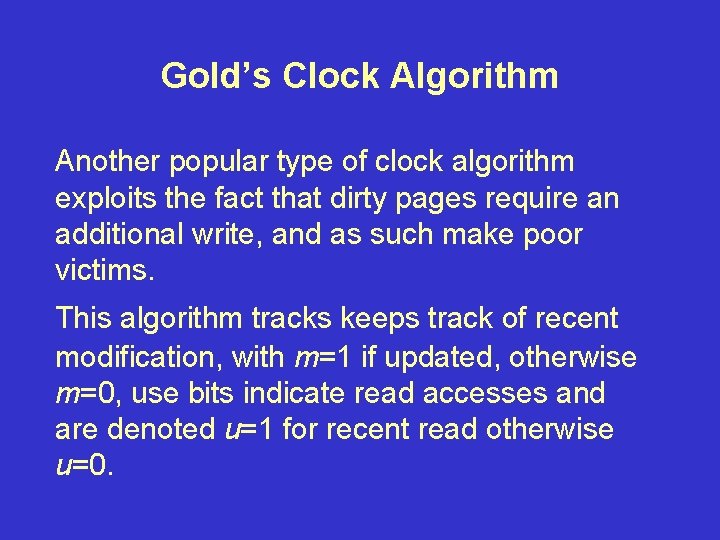
Gold’s Clock Algorithm Another popular type of clock algorithm exploits the fact that dirty pages require an additional write, and as such make poor victims. This algorithm tracks keeps track of recent modification, with m=1 if updated, otherwise m=0, use bits indicate read accesses and are denoted u=1 for recent read otherwise u=0.

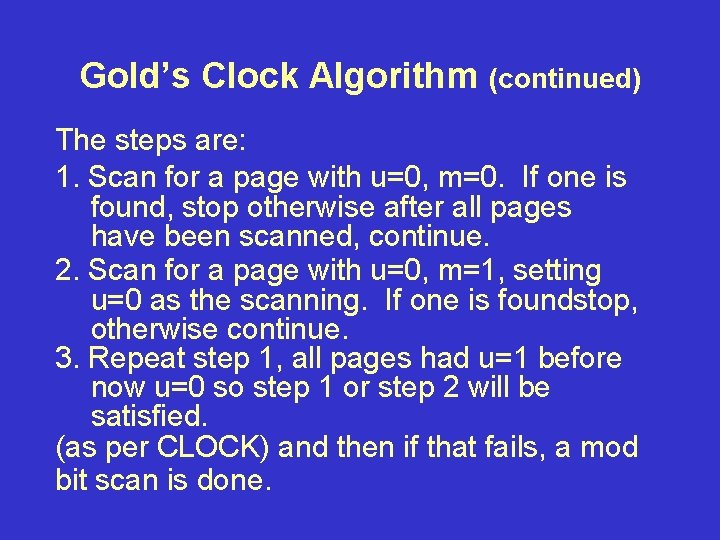
Gold’s Clock Algorithm (continued) The steps are: 1. Scan for a page with u=0, m=0. If one is found, stop otherwise after all pages have been scanned, continue. 2. Scan for a page with u=0, m=1, setting u=0 as the scanning. If one is foundstop, otherwise continue. 3. Repeat step 1, all pages had u=1 before now u=0 so step 1 or step 2 will be satisfied. (as per CLOCK) and then if that fails, a mod bit scan is done.

n 0 P 9 9 P 13 P 47 6 4 P 21 2 4 9 P P 95 P 96 P 9 7 3 5 P 1 Not Accessed 1 recently, modified. P 4 8 P 9 Not Accessed recently, not modified. 7 4 6 5 Accessed recently, not modified.

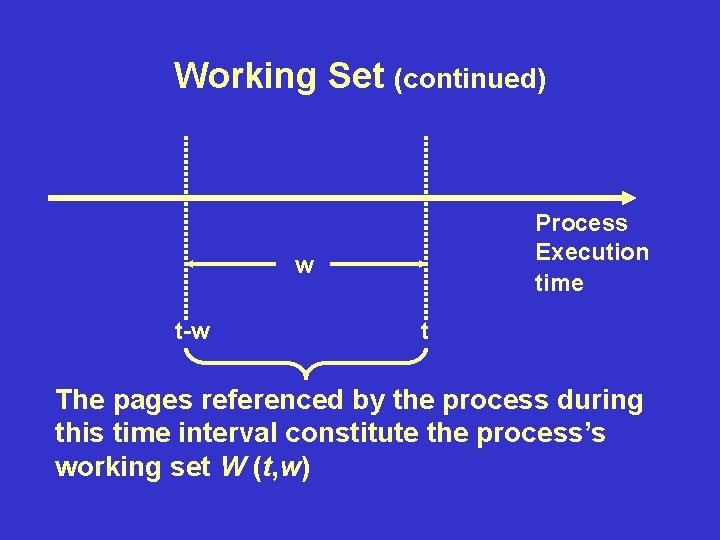
Working Set (WS) Working set algorithms are stack algorithms using a parameter [3, 1]. All pages within the last reference remain resident. The number of pages allocated varies over time (upper bound is ).

Working Set (continued) Process Execution time w t-w t The pages referenced by the process during this time interval constitute the process’s working set W (t, w)

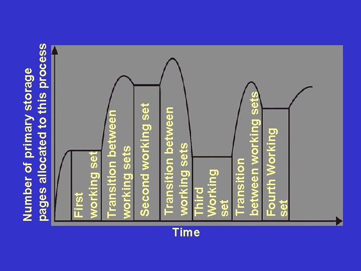
Working Set Characteristics Working sets can be characterized as being stable most of the time, and growing larger as program makes transitions between locals of reference. Choosing or (w) is hard.

Time Transition between working sets Third Working set Transition between working sets Fourth Working set Second working set Transition between working sets First working set Number of primary storage pages allocated to this process

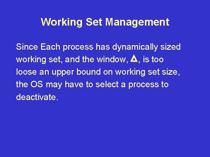
Working Set Management Since Each process has dynamically sized working set, and the window, , is too loose an upper bound on working set size, the OS may have to select a process to deactivate.

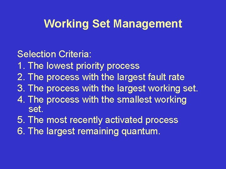
Working Set Management Selection Criteria: 1. The lowest priority process 2. The process with the largest fault rate 3. The process with the largest working set. 4. The process with the smallest working set. 5. The most recently activated process 6. The largest remaining quantum.

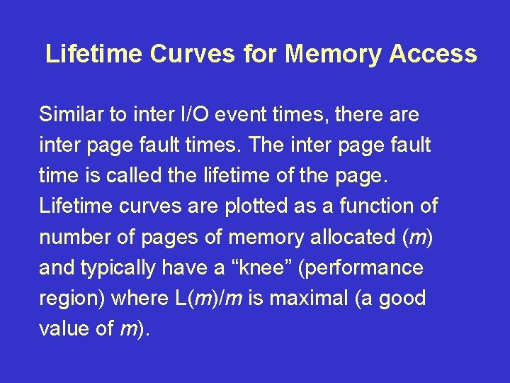
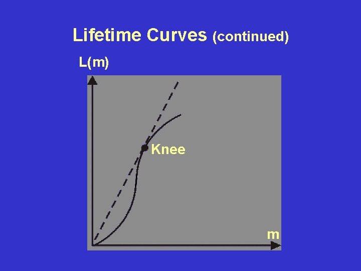
Lifetime Curves for Memory Access Similar to inter I/O event times, there are inter page fault times. The inter page fault time is called the lifetime of the page. Lifetime curves are plotted as a function of number of pages of memory allocated (m) and typically have a “knee” (performance region) where L(m)/m is maximal (a good value of m).

Lifetime Curves (continued) L(m) Knee m

Page Fault Frequency (PFF) Page fault frequency measures the time since the last page and tracks whether each page allocated to a process (via a use bit) has been accessed since the last page fault. This information is used, processes with high fault rates are allocated more pages, while jobs with lower fault rates release pages.