Open vs Closed Loop Frequency Response And Frequency
 Goal: 1) Define")


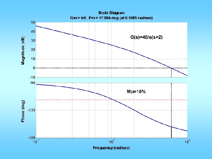
![clear all; n=[0 0 40]; d=[1 2 0]; figure(1); clf; margin(n, d); %proportional control](https://slidetodoc.com/presentation_image_h2/02b692d87bfe8e434045298799bc6ca8/image-12.jpg "clear all; n=[0 0 40]; d=[1 2 0]; figure(1); clf; margin(n, d); %proportional control")
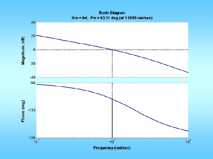
![n=[1]; d=[1/5/50 1/5+1/50 1 0]; figure(1); clf; margin(n, d); %proportional control design: figure(1); hold](https://slidetodoc.com/presentation_image_h2/02b692d87bfe8e434045298799bc6ca8/image-15.jpg "n=[1]; d=[1/5/50 1/5+1/50 1 0]; figure(1); clf; margin(n, d); %proportional control design: figure(1); hold")
 Place wgcd here")
=KP + KDs = KP(1+TDs) • For fixing wgcd and PMd")
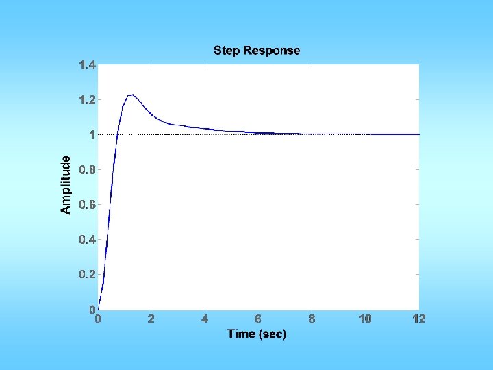
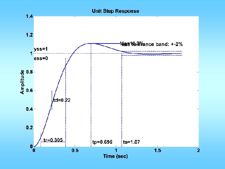
 G(s) Want: maximum overshoot <= 10% rise time <= 0. 3 sec")
![n=[0 0 1]; d=[0. 02 0. 3 1 0]; figure(1); clf; margin(n, d); Could](https://slidetodoc.com/presentation_image_h2/02b692d87bfe8e434045298799bc6ca8/image-29.jpg "n=[0 0 1]; d=[0. 02 0. 3 1 0]; figure(1); clf; margin(n, d); Could")


![n=[0 0 5]; d=[0. 02 0. 3 1 0]; figure(1); clf; margin(n, d); Mp](https://slidetodoc.com/presentation_image_h2/02b692d87bfe8e434045298799bc6ca8/image-35.jpg "n=[0 0 5]; d=[0. 02 0. 3 1 0]; figure(1); clf; margin(n, d); Mp")
![n=[0 0 5]; d=[0. 02 0. 3 1 0]; figure(1); clf; margin(n, d); Mp](https://slidetodoc.com/presentation_image_h2/02b692d87bfe8e434045298799bc6ca8/image-38.jpg "n=[0 0 5]; d=[0. 02 0. 3 1 0]; figure(1); clf; margin(n, d); Mp")
- Slides: 45
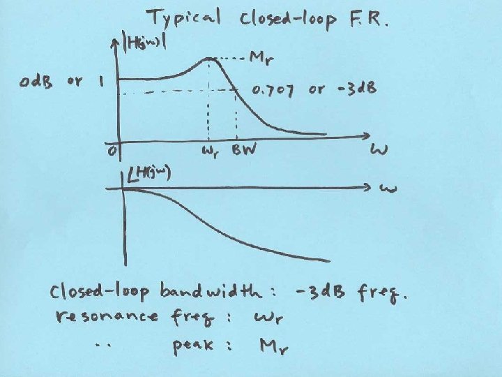
Open vs Closed Loop Frequency Response And Frequency Domain Specifications C(s) Goal: 1) Define typical “good” freq resp shape for closed-loop 2) Relate closed-loop freq response shape to step response shape 3) Relate closed-loop freq shape to open-loop freq resp shape 4) Design C(s) to make C(s)G(s) into “good” shape.
Prototype 2 nd order system closed-loop frequency response z=0. 1 0. 2 0. 3 No resonance for z <= 0. 7 For small zeta, resonance freq is about wn BW ranges from 0. 5 wn to 1. 5 wn For good z range, BW is 0. 8 to 1. 1 wn So take BW = wn Mr=1 d. B for z=0. 6 Mr=3 d. B for z=0. 5 Mr=7 d. B for z=0. 4 w/wn
z=0. 1 0. 2 0. 3 0. 4 wgc In the range of good zeta, wgc is about 0. 65 times to 0. 8 times wn w/wn
z=0. 1 In the range of good zeta, PM is about 100*z 0. 2 0. 3 0. 4 w/wn
Important relationships • Prototype wn, open-loop wgc, closed-loop BW are all very close to each other • When there is visible resonance peak, it is located near or just below wn, • This happens when z <= 0. 6 • When z >= 0. 7, no resonance • z determines phase margin and Mp: z 0. 4 0. 5 0. 6 0. 7 PM Mp 44 25 53 16 61 10 67 5 deg % ≈100 z
Important relationships • wgc determines wn and bandwidth – As wgc ↑, ts, td, tr, tp, etc ↓ • Low frequency gain determines steady state tracking: – L. F. magnitude plot slope/(-20 d. B/dec) = type – L. F. asymptotic line evaluated at w = 1: the value gives Kp, Kv, or Ka, depending on type • High frequency gain determines noise immunity
Desired Bode plot shape
Proportional controller design • Obtain open loop Bode plot • Convert design specs into Bode plot req. • Select KP based on requirements: – For improving ess: KP = Kp, v, a, des / Kp, v, a, act – For fixing Mp: select wgcd to be the freq at which PM is sufficient, and KP = 1/|G(jwgcd)| – For fixing speed: from td, tr, tp, or ts requirement, find out wn, let wgcd = wn and choose KP as above
clear all; n=[0 0 40]; d=[1 2 0]; figure(1); clf; margin(n, d); %proportional control design: figure(1); hold on; grid; V=axis; Mp = 10/100; zeta = sqrt((log(Mp))^2/(pi^2+(log(Mp))^2)); PMd = zeta * 100 + 3; semilogx(V(1: 2), [PMd-180], ': r'); %get desired w_gc x=ginput(1); w_gcd = x(1); KP = 1/abs(polyval(n, j*w_gcd)/polyval(d, j*w_gcd)); figure(2); margin(KP*n, d); figure(3); stepchar(KP*n, d+KP*n);
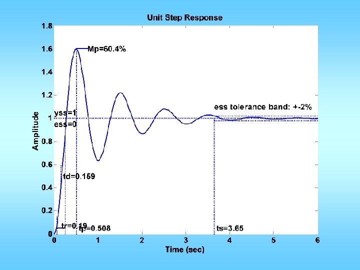
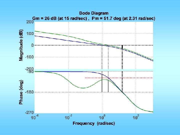
n=[1]; d=[1/5/50 1/5+1/50 1 0]; figure(1); clf; margin(n, d); %proportional control design: figure(1); hold on; grid; V=axis; Mp = 10/100; zeta = sqrt((log(Mp))^2/(pi^2+(log(Mp))^2)); PMd = zeta * 100 + 3; semilogx(V(1: 2), [PMd-180], ': r'); %get desired w_gc x=ginput(1); w_gcd = x(1); Kp = 1/abs(polyval(n, j*w_gcd)/polyval(d, j*w_gcd)); Kv = Kp*n(1)/d(3); ess=0. 01; Kvd=1/ess; z = w_gcd/5; p = z/(Kvd/Kv); ngc = conv(n, Kp*[1 z]); dgc = conv(d, [1 p]); figure(1); hold on; margin(ngc, dgc); [ncl, dcl]=feedback(ngc, dgc, 1, 1); figure(2); step(ncl, dcl); grid; figure(3); margin(ncl*1. 414, dcl); grid;
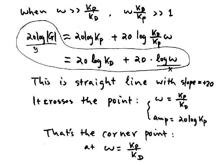
KP/KD 20*log(KP) Place wgcd here
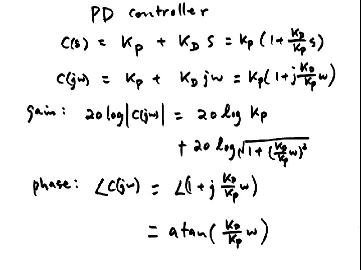
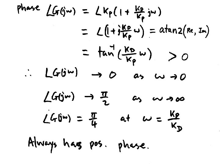
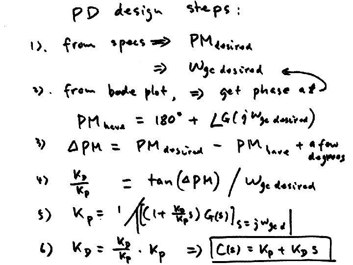
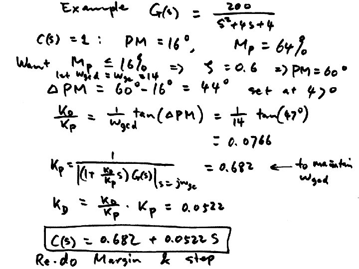
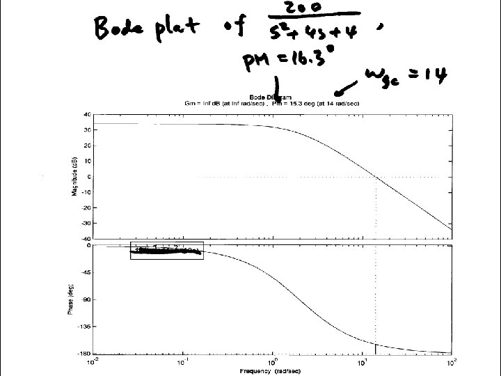
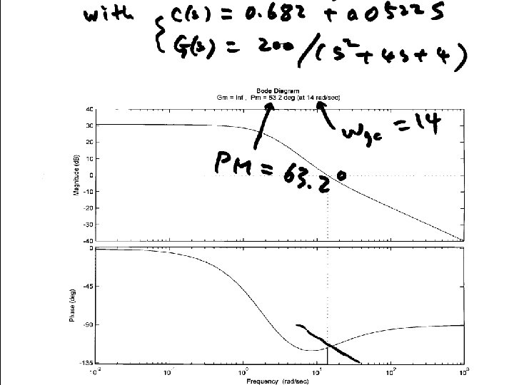
PD Control • C(s)=KP + KDs = KP(1+TDs) • For fixing wgcd and PMd – Compute wgcd from tr, td, etc – Compute PMd from Mp – Compute f = PMd – PM@wgcd – Compute TD = tan(f)/wgcd – KP = 1/sqrt(1+Td 2 wgcd 2)/abs(G(jwgcd)) – KD=KPTD
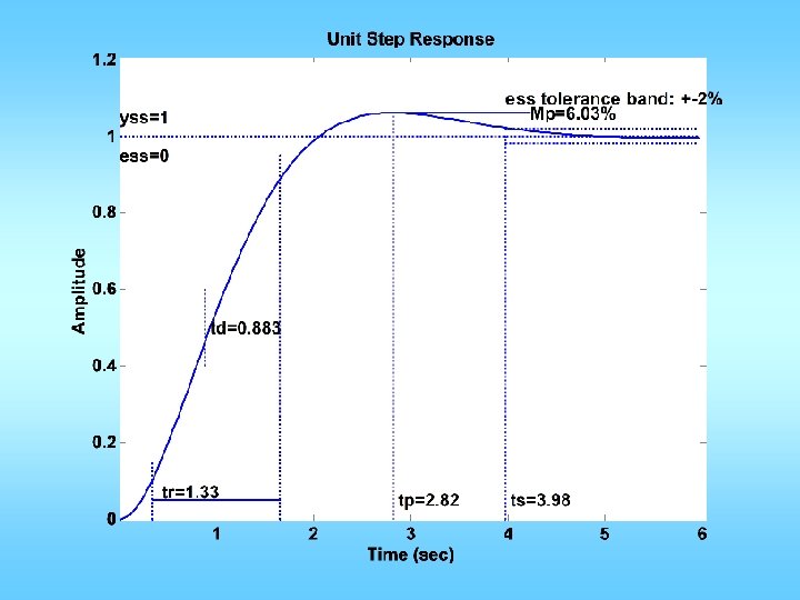
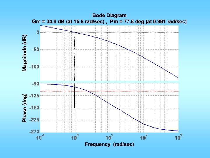
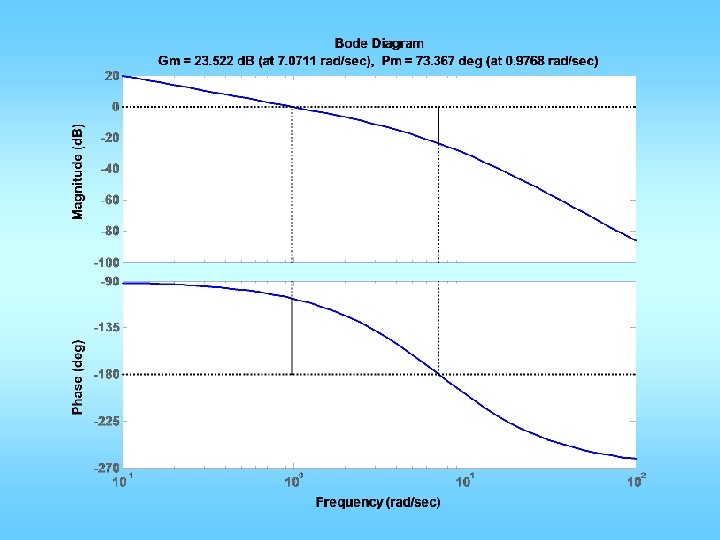
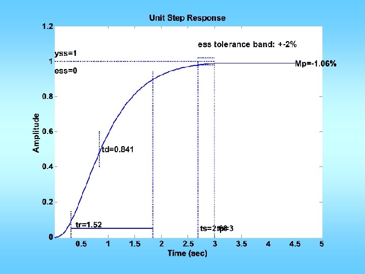
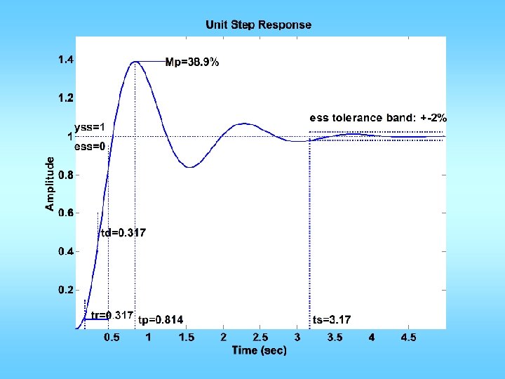
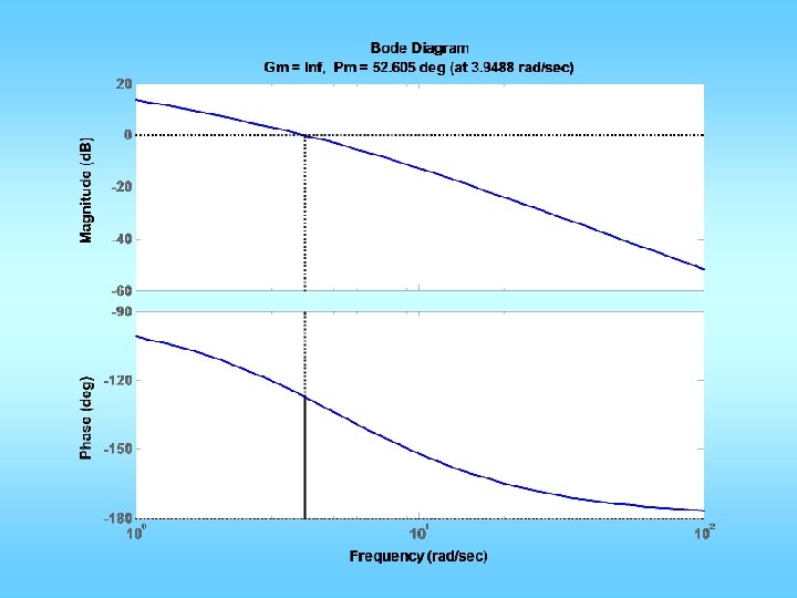
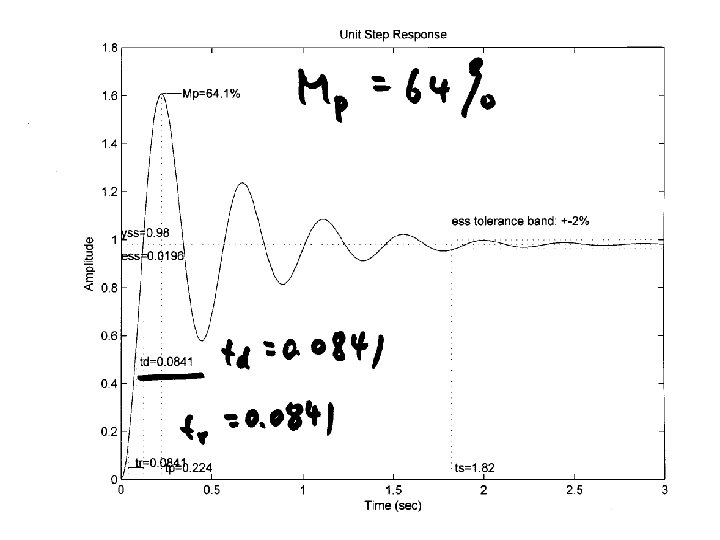
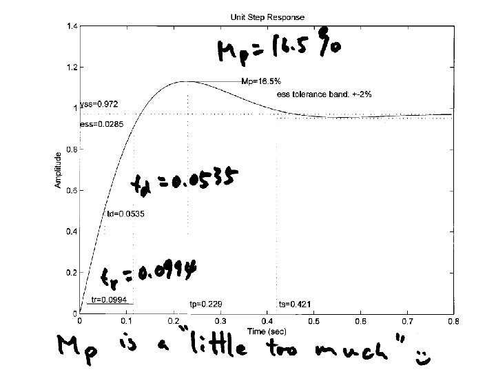
Example C(s) G(s) Want: maximum overshoot <= 10% rise time <= 0. 3 sec
n=[0 0 1]; d=[0. 02 0. 3 1 0]; figure(1); clf; margin(n, d); Could be a little less Mp = 10/100; zeta = sqrt((log(Mp))^2/(pi^2+(log(Mp))^2)); PMd = zeta * 100 + 3; tr = 0. 3; w_n=1. 8/tr; w_gcd = w_n; PM = angle(polyval(n, j*w_gcd)/polyval(d, j*w_gcd)); phi = PMd*pi/180 -PM; Td = tan(phi)/w_gcd; KP = 1/abs(polyval(n, j*w_gcd)/polyval(d, j*w_gcd)); KP = KP/sqrt(1+Td^2*w_gcd^2); KD=KP*Td; ngc = conv(n, [KD KP]); figure(2); margin(ngc, d); figure(3); stepchar(ngc, d+ngc);
Less than spec
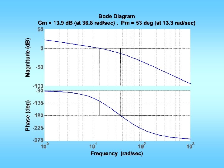
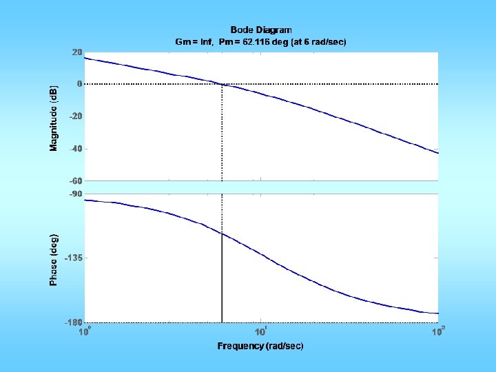
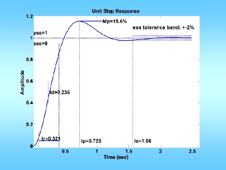
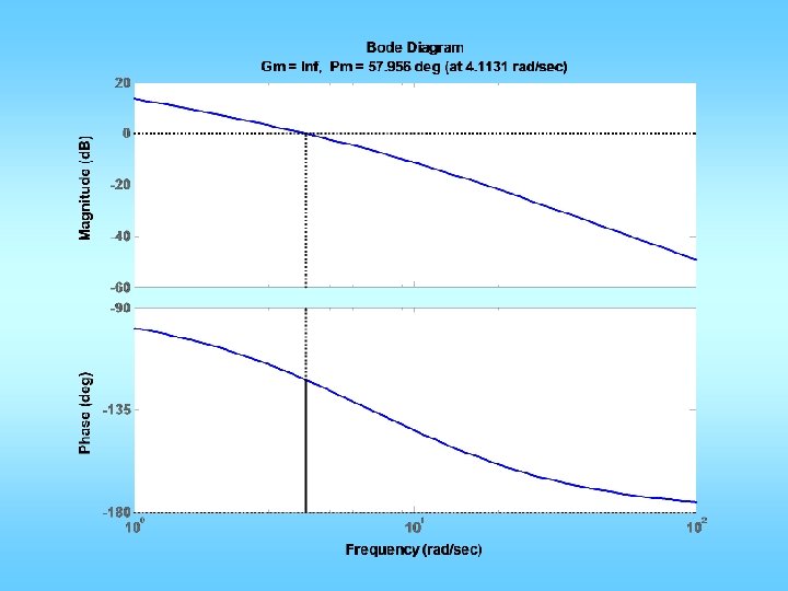
Variation • Restricted to using KP = 1 • Meet Mp requirement • Find wgc and PM • Find PMd • Let f = PMd – PM + (a few degrees) • Compute TD = tan(f)/wgcd • KP = 1; KD=KPTD
n=[0 0 5]; d=[0. 02 0. 3 1 0]; figure(1); clf; margin(n, d); Mp = 10/100; zeta = sqrt((log(Mp))^2/(pi^2+(log(Mp))^2)); PMd = zeta * 100 + 10; [GM, PM, wgc, wpc]=margin(n, d); phi = (PMd-PM)*pi/180; Td = tan(phi)/wgc; KP=1; KD=KP*Td; ngc = conv(n, [KD KP]); figure(2); margin(ngc, d); figure(3); stepchar(ngc, d+ngc);
n=[0 0 5]; d=[0. 02 0. 3 1 0]; figure(1); clf; margin(n, d); Mp = 10/100; zeta = sqrt((log(Mp))^2/(pi^2+(log(Mp))^2)); PMd = zeta * 100 + 18; [GM, PM, wgc, wpc]=margin(n, d); phi = (PMd-PM)*pi/180; Td = tan(phi)/wgc; Kp=1; Kd=Kp*Td; ngc = conv(n, [Kd Kp]); figure(2); margin(ngc, d); figure(3); stepchar(ngc, d+ngc);