Only some part of presentations will be shared

Only some part of presentations will be shared on www. mbchandak. com Email: chandakmb@gmail. com hodcs@rknec. edu

Unit 3 (Part-I): Greedy Algorithms

Expected Outcomes of topic (CO) • Understand problem and its formulation to design an algorithm • Demonstrate the knowledge of basic data structures and their implementation and decide upon use of particular data structure best suited for implementing solution. • Write efficient algorithms using Greedy, Divide & Conquer to solve the real life problems. • Trace logic formulation, execution path of particular algorithm and data generated during execution of algorithm.

Basic Characteristics – Greedy algorithms

Greedy Algorithms • Characteristics • Greedy Algorithms are short – sighted. • Greedy Algorithms are most efficient if it works. • For every instance of input Greedy Algorithms makes a decision and continues to process further set of input. • The other input values at the instance of decision are lost and not used in further processing. 5 A 8 5 S D t y 9 B x 2 S A 8 D

Greedy Algorithm: Knapsack Problem • Principle: Knapsack is a bag of fixed capacity. • In this problem it is assumed that “n” objects with profit value and weight are given. • The main objective is to select the objects and place them in knapsack such that the object placed in the bag will generate maximum profit. • Two types of Knapsack problems: • Fractional Knapsack problem • 0/1 Knapsack problem • The Fractional Knapsack problem can be solved using Greedy approach, where as 0/1 Knapsack problem does not have greedy solution.

Representation Capacity = 20 10/2 9/4 15/3 6/6 4/1 11/5

Greedy Algorithm: Knapsack Problem • Approaches: • There are three basic approaches to solve knapsack problem: • Select the maximum profit objects • Select the minimum weight objects • Select the objects based on Profit/Weight ratio

Significance TIME PROFIT Process for execution Generate maximum Profit in available time by proper selection of processes

Greedy Algorithm: Knapsack Problem Example 1: Capacity = 15, number of objects = 7 Profit Weight Index 10 2 5 3 15 5 7 7 6 1 18 4 3 1 1 2 3 4 5 6 7 Approach: Maximum Profit Object Weight Profit Capacity Remaining Partial/Complete O 6 4 18 15 -4=11 C O 3 5 15 11 -5=6 C O 1 2 10 6 -2=4 C O 4* 4 4 4 -4=0 P TOTAL 15 47 0

Greedy Algorithm: Knapsack Problem Example 1: Capacity = 15, number of objects = 7 Profit Weight Index 10 2 5 3 15 5 7 7 6 1 18 4 3 1 1 2 3 4 5 6 7 Approach: Minimum Weight Object Weight Profit Capacity Remaining Partial/Complete O 5 1 6 15 -1=14 C O 7 1 3 14 -1=13 C O 1 2 10 13 -2=11 C O 2 3 5 11 -3=8 C O 6 4 18 8 -4=4 C O 3* 5(4) 12 4 -4=0 P TOTAL 15 54 0

Greedy Algorithm: Knapsack Problem Example 1: Capacity = 15, number of objects = 7 Profit Weight Ratio Index 10 2 5 3 15 5 7 7 6 1 18 4 3 1 5. 0 1. 6 3. 0 1. 0 6. 0 4. 5 3. 0 1 2 3 4 5 6 7 Approach: Maximum Pi/Wi ratio Object Weight Profit Capacity Remaining Partial/Complete O 5 1 6 15 -1=14 C O 1 2 10 14 -2=12 C O 6 4 18 12 -4=8 C O 3 5 15 8 -5=3 C O 7 1 3 3 -1=2 C O 2* 3(2) 10/3=3. 33 2 -2=0 P TOTAL 15 55. 3 0

Greedy Algorithm: Knapsack Problem Example 2: Capacity = 18, number of objects = 7 Pi Wi 9 2 15 3 12 5 4 4 6 3 16 6 8 3 Ratio 4. 5 5. 0 2. 4 1. 0 2. 6 Index 1 2 3 4 5 6 7 Maximum (Pi/Wi) Ratio Object Weight Profit Capacity Remaining Partial/Complete

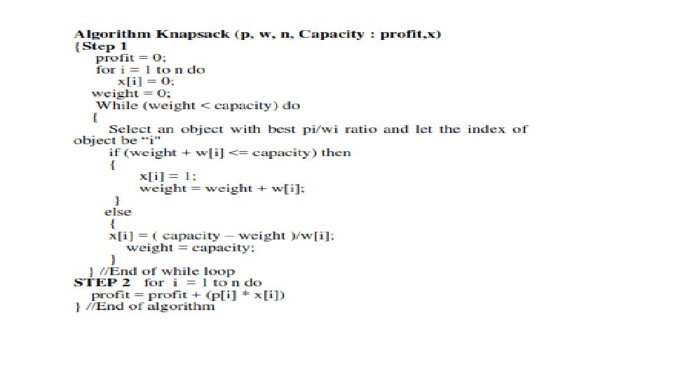
Knapsack Problem: Algorithm • Data Structures: • Weight array: W[n] To store weight values • Profit array: P[n] To store profit values • Capacity Given and will decrease after each step • X[n] To store 0, 1 or fraction depending upon object placement • Weight = 0 (initially) and will increase towards capacity • Profit = 0 and will be calculated by X[i] and P[i] • Process: To select the object with best Pi/Wi Ratio. (Sorting)

Knapsack Algorithm • Initialization steps: • Profit • Weight • x[1. . n] to hold data about object placement [partly, completely, rejected] • Decision step • While ( condition ) • Select object //Call function for selecting best suited object// • Place in bag {Completely / Partially } • Update x [i] • Final step: Find profit • Multiply x[i] and associated profit

Greedy Algorithms on Graph Prim’s Algorithm Kruskal Algorithm Single Source shortest Path Algorithm (Dijkstra’s Algorithm)

Minimum Cost Spanning Tree • Given a graph G =(V, E) V=Number of vertices and E=Number of edges, then Spanning tree is tree generated from graph, with characteristics • All the vertices present in the tree • There is no cycle in the tree i. e. , e=v-1 • Subset of edges, that forms a tree, where total cost of edges is minimum. • Minimum cost spanning tree is a spanning tree with “edges of minimum cost”. • Applications: • To transmit the message without broadcasting. • To generate travel plan in minimum cost. • Designing network, home electric wiring etc. • Approaches: Prims’ Method and Kruskals’ Method.

Minimum Cost Spanning Tree • Principle: • Select an edge of minimum cost. The edge will derive two vertices. • Continue the process from one of the vertex by selecting the next edge of minimum cost. • Once the vertex is visited, then it is marked. • The process will attempt to visit unmarked vertices and terminates when all the vertices are visited. • Process guarantees no cycle in the tree. • “What if the process of tree generation starts from any arbitrary vertex”. • Motivation: To join points as cheaply as possible: Applications in clustering and networking • Acyclic graph to connect all nodes in minimum cost. • One of the term in U. S. legal code (AT&T)

Graphs for Examples Steiner Spanning Tree

Spanning tree: Free tree • A free tree has following properties 1. Exactly n-1 edges for “n” vertices 2. There exists a unique path between two vertices. 3. By adding an edge, a cycle will be created in free tree. Breaking any edge on the cycle restores the free tree. • Greedy: Minimization problem. 1. Repeated selection: of minimum cost edges with certain test cases. 2. Once decision of adding edge is finalized, it cannot be revoked. 3. Basic idea: To generate subset of “E” connecting all “V”

Minimum Cost Spanning Tree: Prim’s method • Example: • Consider the following graph: 1 10 2 45 30 4 20 25 6 50 40 5 55 3 35 15 • Select an edge of minimum cost. • From selected vertex continue selecting edge of minimum cost 1 2 3 4 5 6 1 99 10 99 30 45 99 2 10 99 50 99 40 25 3 99 50 99 99 35 15 4 30 99 99 20 5 45 40 35 99 99 55 6 99 25 15 20 55 99 2 1 3 4 5 6

Minimum Cost Spanning Tree: Prim’s method • Example: • Consider the following graph: 10 1 2 45 30 40 25 4 20 50 6 5 2 3 4 5 6 1 99 10 99 30 45 99 2 10 99 50 99 40 25 3 99 50 99 99 35 15 4 30 99 99 20 The next vertex should be the vertex reachable in 5 45 40 from 35 vertex 99 99 2 55 minimum cost either 1 or vertex 6 99 25 15 20 55 99 3 35 55 1 10 2 T C F 1 1 - 1 2 2 1 - 2 2 R 1 2 3 4 5 6 3 1 < 3 2 F - - 2 1 2 2 4 1 < 4 2 T 5 1 < 5 2 F 6 1 < 6 2 F Out of Four possible options: cost[near[j], j] = minimum Select the index satisfying above condition: 6

Minimum Cost Spanning Tree: Prim’s method The vertex selected is “ 6” due to which there may be changes in closeness of vertices. That the vertices which were close to vertex 1 or vertex • Example: 2 may modified due to selection of vertex 6. • Consider the following graph: 10 1 2 45 30 40 25 4 20 50 6 5 3 35 55 2 3 4 5 - - 6 6 2 2 3 4 5 6 1 99 10 99 30 45 99 2 10 99 50 99 40 25 3 99 50 99 99 35 15 4 30 99 99 20 5 45 40 35 99 99 55 6 99 25 15 20 55 99 T 15 1 10 2 6 1 Out of 2 Four possible 3 4 5 cost[near[j], j] 6 options: = minimum 3 - Select -the index 2 satisfying 1 above 2 condition: 2 25 6 C 1 - 1 2 - 2 F R 3 6 < 3 2 T 4 1 < 4 6 F 5 6 < 5 2 F - 6 6

Minimum Cost Spanning Tree: Prim’s method The vertex selected is “ 3” due to which there may be changes in closeness of vertices. That the vertices which were close to vertex 1 or vertex • Example: 2 or vertex 6 may modified due to selection of vertex 3. • Consider the following graph: 10 1 45 30 - 2 3 - 20 - 50 40 25 4 1 2 4 66 5 5 55 3 3 35 1 2 3 4 5 6 1 99 10 99 30 45 99 2 10 99 50 99 40 25 3 99 50 99 99 35 15 4 30 99 99 20 5 45 40 35 99 99 55 6 99 25 15 20 55 99 6 - 1 2 3 4 5 6 - - 6 6 2 - T 15 1 1 Out of 2 Four possible 3 4 5 cost[near[j], j] 6 options: = minimum 4 - Select -the index 2 satisfying 1 above 2 condition: 2 10 2 25 6 15 3 C 1 - 1 2 - 2 3 < 3 F R 4 3 < 4 6 F 5 3 < 5 2 T - 6 6

Minimum Cost Spanning Tree: Prim’s method The vertex selected is “ 4” due to which there may be changes in closeness of vertices. That the vertices which were close to vertex 1, 2, 6, 3 may • Example: modified due to selection of vertex 4. • Consider the following graph: 10 1 1 2 - - 1 2 3 - 20 - 3 30 4 - - 45 4 25 4 66 2 5 50 40 6 3 5 - 5 6 55 3 3 35 - 1 2 3 4 5 6 - - 6 6 2 - 1 2 3 4 5 6 - - 2 1 2 3 4 5 6 1 99 10 99 30 45 99 2 10 99 50 99 40 25 3 99 50 99 99 35 15 4 30 99 99 20 5 45 40 35 99 99 55 6 99 25 15 20 55 99 T 15 10 1 2 25 4 6 20 15 3 C F 1 - 1 2 - 2 3 < 3 4 < 5 - 6 5 6 3 R F 4 T

Prim’s method: Output • Example: • Consider the following graph: 1 10 2 45 30 4 20 25 6 50 40 5 55 3 35 15 1 2 3 4 5 6 1 99 10 99 30 45 99 2 10 99 50 99 40 25 3 99 50 99 99 35 15 4 30 99 99 20 5 45 40 35 99 99 55 6 99 25 15 20 55 99 Vertex 1 Vertex 2 Cost 1 2 10 2 6 25 6 3 15 6 4 20 3 5 35 TOTAL 105

Algorithm: Prim’s Algorithm • Data Structures: Input • cost[1. . n, 1. . n] To store the cost information • Intermediate: • near[1. . n] To store near information for selected vertex • Output: • mincost=0 • t[1. . n-1, 1. . 3] To store the spanning tree

Algorithm Prim(cost, n: mincost, t) { Step 1: Select an edge of minimum cost from the cost matrix and let it be cost[k, l] mincost = cost[k, l]; t[1, 1] = k; t[1, 2] = l; t[1, 3] = cost[k, l] for 1 = 1 to n do { if cost[i, l] < cost[i, k] then near[i] = l; else near[i] = k; } //end of for i = 2 to n-1 do { let j be an index such that (near[j] ≠ 0 and cost[near[j], j] = minimum) t[i, 1] = j; t[i. 2] = near[j] t[i, 3] = cost[near[j], j] near[j] = 0; for k = 1 to n do if((near[k] ≠ 0) and cost[k, near[k] > cost[k, j])) near[k] = j; } //End of for } //End of algorithm

Minimum Cost Spanning Tree: Prim’s Algorithm • Designed by Robert C. Prim in 1957 and was modified by Dijkstra so also called as DJP algorithm.

Proof of Correctness: Prims’ Algorithm • The proof of prims’ algorithms is described using CUT property of a graph. • Let G=(V, E) be the graph, then CUT property will divide the graph into two sets of vertices (X and V-X), such that there exists three types of edges. • Edges with both vertices in “X” • Edges with both vertices in “V-X” • Edges with one vertex in “X” and one vertex in “V-X” Crossing edge • If there are “n” vertices in graph, then number of cuts will be 2 n • Empty cut lemma: • A graph is said to be not connected, if cut has no crossing edges. This is denoted as empty cut. • The correctness is proved using straight forward induction method.

Minimum Cost Spanning Tree: Kruskals’ Algorithm • Principle: Select an edge of minimum cost. At each step add a new edge with next minimum cost to graph, such that it does not generate cycle. • Kruskals’ algorithm, grows like forest and then generates a tree. • Integration plays major role. • Implementation: • From the set of edges, select an edge of minimum cost • Again continue the process with an edge of next minimum cost, add edge if not generating cycle.

Kruskals’ Algorithm • Process-1: To find an edge of minimum cost • Sort the edges in ascending order of weight: O(e * log e) • Process-2: To check by adding an edge cycle is generated. • Union-Find Data structure is used to check if cycle is generated. • The algorithm creates set for each vertex: [1] [2] [3] [4] [5] [6] etc. • When an edge [u, v] is selected Find[u] will return the set in which vertex “u” is present and Find[v] will return the set in which vertex “v” is present. • If returned set are distinct, then edge can be added and sets can merged.

Kruskals’ Algorithm: Example

Kruskals’ Algorithm • Example:

Kruskals’ Algorithm: Implementation • Table for generating tree: Edge Cost Action Component [1] [2] [3] [4] [5] [6] [7] (1, 2) (2, 3) (4, 5) (6, 7) (1, 4) (2, 5) (4, 7) 1 2 3 3 4 4 4 Accept Accept Reject Accept [1, 2] [3] [4] [5] [6] [7] [1, 2, 3] [4, 5] [6, 7] [1, 2, 3, 4, 5, 6, 7]

Algorithm

Complexity of Kruskals algorithm • Let “E” be number of edges in the graph and “n” be number of vertices in the graph. • To Sort “E” edges, the time requirement will be O(E log E) which can be further reduced to O(E log n) since n-1 < E < n(n-1)/2 • For creating the vertex set time required will be O(V) • For finding the vertex set of V 1 and V 2 and merging if the set is distinct, time required will be O(E log n) • Thus the complexity of Kruskals algorithm will be O(E log n)

Practice examples

Single Source Shortest Path • An approach to find shortest path from given source vertex to all possible destinations. • Minimization problem: To find the path of minimum cost • Path may be direct or indirect • Various algorithms: • Dijkstra’s algorithm can be used if no negative edges are present. • Bellman Ford algorithm can be used if negative edges are present. • Floyd’s and Warshall’s algorithm is extension and called as all pair shortest path algorithm, if no negative edges are given.

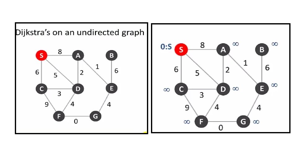
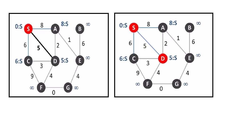
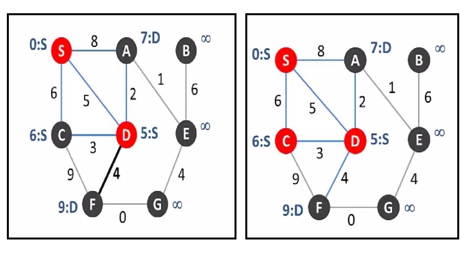
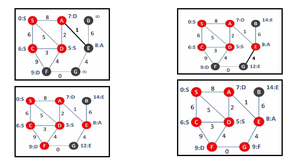
Example: Dijkstra’s Algorithm 55 55 25 45

Example: Dijkstra’s Algorithm B A 20 Fix(B) B - F C D E F 80 - - 90 - 10=>30 Fix(F) Source B 20: A-B F 30: A-B-F C 80: A-B-F-C D 90: A-B-F-C-D H 100: A-B-F-C-H G 110: A--G - 50=>20 - - G E - 50=>10 Fix (D) D A H 30=>50 Fix(F) C H G Not Reachable - - -

Example: Single source shortest path 0 1 2 3 4 5

Algorithm: Data Structures • • • Input: Cost matrix [nxn] and source vertex Intermediate: s[1. . n] to store information about reached vertices Parent[1. . n] is used to hold information about the parent node from which the desired node is reachable. Output: dist[1. . n] and parent[1. . n] Process: Initially the vertex at minimum distance from the source is selected. The reachable vertices from source vertex are also initially selected. When new vertex is added in the reachable list, the existing paths and paths generated from reached vertex are compared to make the next decision.

Single Source Shortest Path: Algorithm

Job Scheduling: Without Deadline • Principle: • This application is related with execution of jobs on the system in such a way that – • Average time spent by the jobs with machine is minimum • To maximize the profitability by completing the job before deadline. • In banks, where large number of transactions is taking place, it is required to complete the transaction in stipulate time period. If transaction are more and there is only one processor, then the transactions are buffered, but the execution should be so managed that average time spent by transaction in buffer is minimized.

Job Scheduling: Without Deadline • Implementation: Shift the shorter jobs ahead of longer jobs • P 1 = 4, P 2 = 6, P 3 = 3, P 4 = 8 and P 5 = 2 Find the minimal time required to service the customers • Solution: • Rearrange in the ascending order to time requirement: • P 5 = 2, P 3 = 3, P 1 = 4, P 2 = 6 and P 4 = 8 Formulation: N * t 1 + (N-1) * t 2 + (N-2) * t 3 + (N-3) * t 4 + (N – (N-1)) * tn

Job Scheduling without Deadline • Principal: Given set of “n” jobs. • To decide the schedule, so as to complete the job processing in minimum time. • To prove the approach is correct. • Method: SJF: Shortest Job First • Select the job with minimum time requirement and process. Delay the jobs with higher time requirements. • Process required: Sorting of Jobs. • Note: All the jobs present in the set will be executed.

Example Total number of jobs=6 Job 1 2 3 4 5 6 Time 12 8 3 9 4 6 Job 1 2 3 4 5 6 Time 3 4 6 9 8 12 Index 1 2 3 4 5 6 • Total processing time: (3 x 6) + (4 x 5) + (6 x 4) + (9 x 3) + (8 x 2) + (12 x 1) =

Job Scheduling with Deadline • Principal: Given set of “n” jobs. • To decide the schedule, so as to complete the job processing in minimum time. • Each job requires only one cycle for execution. • With each job deadline and profit is associated. • The profit is valid till the deadline. • Process required: Sorting of Jobs. • Note: Does not guarantee the execution of all the jobs present in the set.

Example Find the maximum value of deadline This will provide details about maximum cycles available for execution For example: Maximum value of deadline = 7 Hence there can be SEVEN slots for execution each of size ONE UNIT Step 1: Sort the jobs on maximum value of profit Step 2: Allocation of slot on maximum deadline basis Step 3: Job rejection process

Example. . • After sorting Slot Task / Profit 1* T 2/20 2 T 7/23 3 T 9/25 4 T 5/18 5 T 3/30 6* T 1/16 7 T 8/16 Total Profit

Unit 3: Part II: Divide and Conquer • Principle: • Input is divided into small groups before processing using logical division. • Solution space for all the divided groups is same and unique. • The CPU utilization is on higher side whereas the throughput is on lower side. • The division of input reduces the complexity of the process and most of DAC based algorithms have logarithmic complexity. • DAC principle is mostly applied for input of large size.

Binary Search •

Binary Search: Numerical on average number of comparisons for successful and unsuccessful search • Consider the following array of size: 14 (1. . 14 low=1 and high=14) I 1 2 3 4 5 6 7 8 9 10 11 12 13 A -10 -5 7 14 21 34 45 56 65 77 89 98 104 110 C 3 4 2 4 3 4 1 4 3 4 2 4 3 14 4 • Total number of comparisons for successful search: 43 • Average number of comparisons = 43/14 = 3. 07 • For finding total number of comparisons for unsuccessful search: • Draw Binary search tree for the given array • Complete the BST and find the sum of level of BST • Compute average by dividing the sum/n+1 (where n = number of elements)

Binary Search: Numerical on average number of comparisons for successful and unsuccessful search I 1 2 3 4 5 6 7 8 9 10 11 12 13 A -10 -5 7 14 21 34 45 56 65 77 89 98 104 110 C 3 4 2 4 3 4 1 4 3 4 2 4 3 14 4

Binary Search: Algorithm and complexity equation • Algorithm Binary. Search(a, i, l, x) //x is the element to be searched { If(i==l) then { If(x=a[i]) return(i); else return(0); } Else { Mid=[i+l]/2 If(x==a[mid]) then Return(mid) Else If(x<a[mid])then Return (bsearch(a, i, mid-1, x) Else Return (bsearch(a, mid+1, l, x); }

Ternary Search

Sorting algorithms: Merge Sort • Basis: • Split phase • Divide the array into smaller units: of size 1. • Merge phase • Compare the two adjacent elements, sort elements and merge to generate array at next level. Continue merge process till all units are merged into single unit. There are various methods to perform split operation. Divide the array at each element (Cutting the long piece of cake), will require n 1 operations. Otherwise apply logarithmic division: divide by 2 option. This will require log n operations.

Merge Sort: Example SPLIT PHASE L 1 L 2 L 3 MERGE PHASE

Merge Sort Algorithm and Complexity Equation • There are two components in merge sort: split and merge Algorithm Merge_Sort(a, low, high) { if(low<high) { Complexity Equation: T(n) = 2 T(n/2) + n mid= low+high/2 For division by factor 2, and two recursive calls Time required = 2 T(n/2) Merge_Sort(a, low, mid) For merging “n” elements time required = n Merge_Sort(a, mid+1, high) Merge(a, low, high) } }

Merge Sort Algorithm: Characteristics • Merge sort requires auxiliary array for storing the sorted elements after every merge phase. • Discuss time complexity.

Min-Max Algorithm • Principle: Method to find minimum and maximum element from an array. • General method requires 2*(n-1) comparisons. Algorithm min_max(a, n, min, max) { min = max = a[1] for i = 2 to n do { if (a[i] < min) then min = a[i] if (a[i] > max) then max = a[i] } }

Min-Max: DAC based Example 1 2 3 4 5 6 7 8 9 10 22 13 -5 -8 15 60 17 31 47 45 1 2 3 4 5 6 7 8 1 2 3 6 7 8 13 22 -5 17 60 31 4 9 10

Min-Max: DAC Algorithm min_max(a, i, j, min, max) { If (i==j) then min=max=a[i] Else If(i=j-1) then { if(a[i] < a[j]) then { min = a[i]; max=a[j] } else { min=a[j]; max=a[i] } Else { mid = [i+j] / 2 (Take lower integer) min_max(a, i, mid, min, max) min_max(a, mid+1, j, min 1, max 1) if (max < max 1) then max = max 1 if (min > min 1) then min = min 1 } } • • Complexity equation: T(n) = T(n/2) + 2 for n > 2 T(n) = 1 if n=2 T(n) = 0 if n=1

Quick Sort Analysis Algorithm Quick. Sort(a, start, end) { If (start < end) C 1 { X = partition(a, start, end) Check partition time Quicksort(a, start, x-1) T(n/2) Quicksort(a, x+1, end) T(n/2) } } Total time including partition = 2 T(n/2) + an + b + c 1 2 T(n/2) + an Which can be written as: 2 T(n/2) + cn, where c = constant. If there is only one element, then T(1) = c, because “if” loop will not be executed.

Quick Sort Analysis Algorithm partition(a, start, end) { pivot = a[end]; pindex = start; for i = start to end-1 do { if (a[i] <= pivot) { swap(a[i], a[pindex]) pindex++; } swap(a[pindex], pivot) return(pindex) } Total time = an+b 1 unit “a” time unit for “n” times 1 unit

Mathematical solving •

Worst Case • In worst case the given array is already sorted and it is required to sort it in reverse order. (ascending to descending). • Next into 1 time the 2 array will 3 be partitioned 4 5 two un-balanced 6 7 partitioned. 8 • And in all steps, the resultant arrays will be un-balanced. • In such case: the second Quicksort function will not be executed and time complexity will be controlled by only first quicksort function. This function will be executed for T(n-1) times. • T(n) = T(n-1) + cn • T(n) = T(n-2) + c(n-1) + cn = T(n-2) + 2 cn – c • T(n) = T(n-3) + c(n-1) + 2 cn – c • T(n-3) + c(n-2) + 2 cn – c = T(n-3) + 3 cn – 3 c • T(n-4) + 4 cn – 6 c • T(n-k) + kcn – (k(k-1)/2) • Smallest unit = n-k= 1, hence k = n ignoring the constants. • T(n) = T(1) + ncn – constant term nxn = n 2