Online Convex Optimization with TimeVarying Constraints 1 2

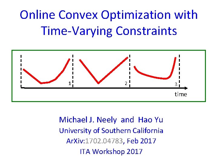
Online Convex Optimization with Time-Varying Constraints 1 2 3 time Michael J. Neely and Hao Yu University of Southern California Ar. Xiv: 1702. 04783, Feb 2017 ITA Workshop 2017

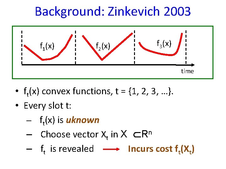
Background: Zinkevich 2003 f 1(x) f 2(x) f 3(x) time • ft(x) convex functions, t = {1, 2, 3, …}. • Every slot t: – ft(x) is uknown – Choose vector Xt in X Rn – ft is revealed Incurs cost ft(Xt)

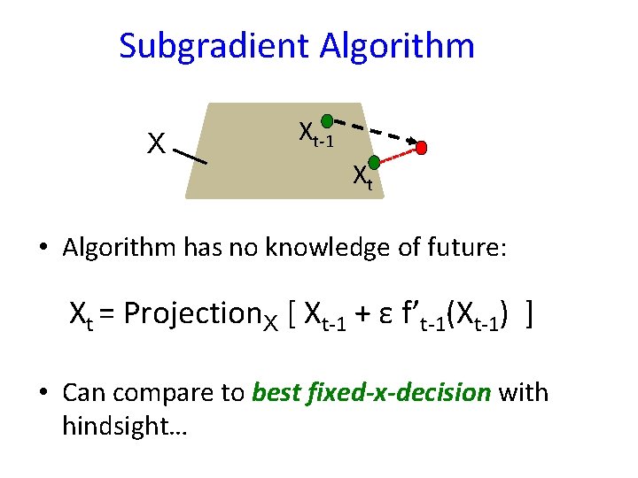
Subgradient Algorithm X Xt-1 Xt • Algorithm has no knowledge of future: Xt = Projection. X [ Xt-1 + ε f’t-1(Xt-1) ] • Can compare to best fixed-x-decision with hindsight…

Zinkevich Result [2003] • ε-approx with convergence time 1/ε 2: For any fixed x* in X we have • O( T ) regret:

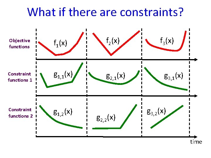
What if there are constraints? Objective functions f 1(x) f 2(x) Constraint functions 1 g 1, 1(x) g 2, 1(x) Constraint functions 2 g 1, 2(x) g 2, 2(x) f 3(x) g 3, 1(x) g 3, 2(x) time

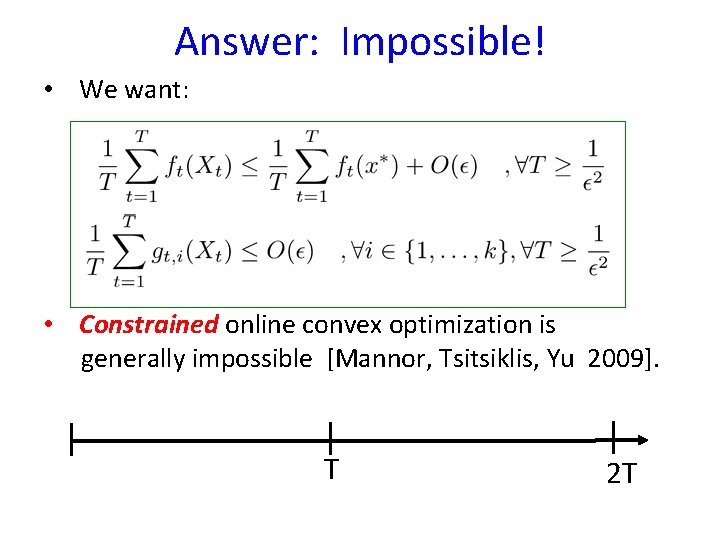
Answer: Impossible! • We want: • Constrained online convex optimization is generally impossible [Mannor, Tsitsiklis, Yu 2009]. T 2 T

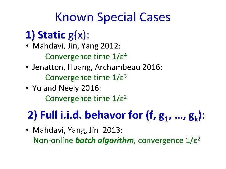
Known Special Cases 1) Static g(x): • Mahdavi, Jin, Yang 2012: Convergence time 1/ε 4 • Jenatton, Huang, Archambeau 2016: Convergence time 1/ε 3 • Yu and Neely 2016: Convergence time 1/ε 2 2) Full i. i. d. behavor for (f, g 1, …, gk): • Mahdavi, Yang, Jin 2013: Non-online batch algorithm, convergence 1/ε 2

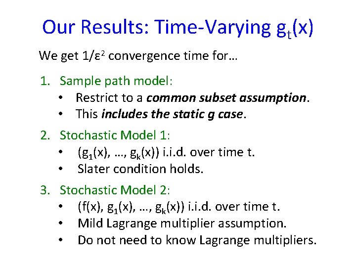
Our Results: Time-Varying gt(x) We get 1/ε 2 convergence time for… 1. Sample path model: • Restrict to a common subset assumption. • This includes the static g case. 2. Stochastic Model 1: • (g 1(x), …, gk(x)) i. i. d. over time t. • Slater condition holds. 3. Stochastic Model 2: • (f(x), g 1(x), …, gk(x)) i. i. d. over time t. • Mild Lagrange multiplier assumption. • Do not need to know Lagrange multipliers.

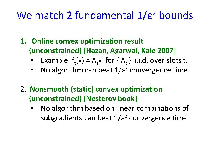
We match 2 fundamental 1/ε 2 bounds 1. Online convex optimization result (unconstrained) [Hazan, Agarwal, Kale 2007] • Example ft(x) = Atx for { At } i. i. d. over slots t. • No algorithm can beat 1/ε 2 convergence time. 2. Nonsmooth (static) convex optimization (unconstrained) [Nesterov book] • No algorithm based on linear combinations of subgradients can beat 1/ε 2 convergence time.

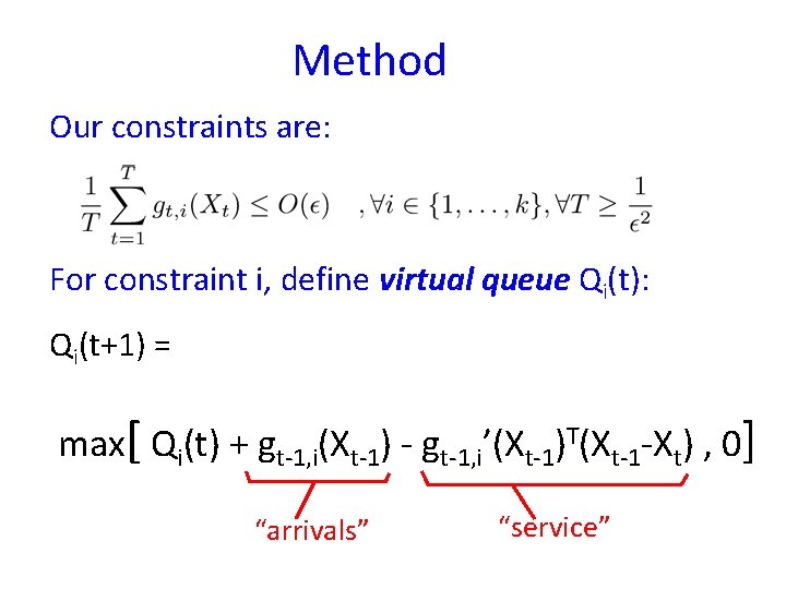
Method Our constraints are: For constraint i, define virtual queue Qi(t): Qi(t+1) = max[ Qi(t) + gt-1, i(Xt-1) - gt-1, i’(Xt-1)T(Xt-1 -Xt) , 0] “arrivals” “service”

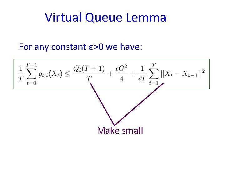
Virtual Queue Lemma For any constant ε>0 we have: Interpretation…

Virtual Queue Lemma For any constant ε>0 we have: Make small

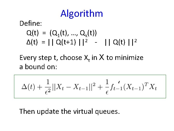
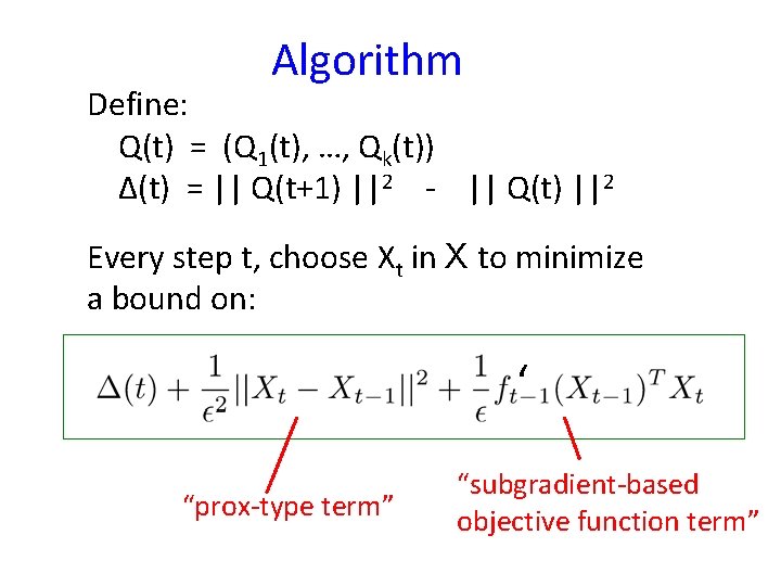
Algorithm Define: Q(t) = (Q 1(t), …, Qk(t)) Δ(t) = || Q(t+1) ||2 - || Q(t) ||2 Every step t, choose Xt in X to minimize a bound on: ‘ Then update the virtual queues.

Algorithm Define: Q(t) = (Q 1(t), …, Qk(t)) Δ(t) = || Q(t+1) ||2 - || Q(t) ||2 Every step t, choose Xt in X to minimize a bound on: ‘ “prox-type term” “subgradient-based objective function term”

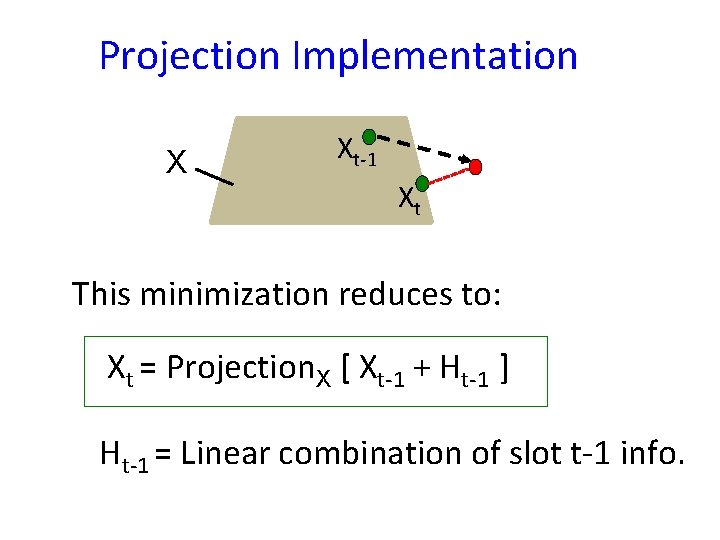
Projection Implementation X Xt-1 Xt This minimization reduces to: Xt = Projection. X [ Xt-1 + Ht-1 ] Ht-1 = Linear combination of slot t-1 info.

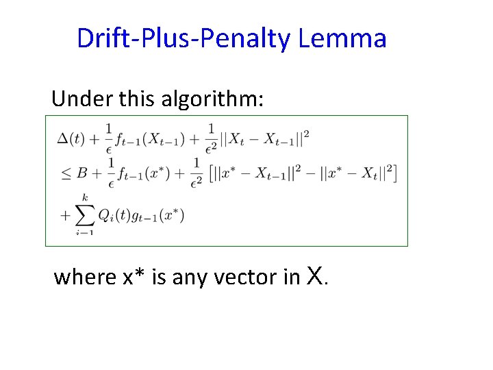
Drift-Plus-Penalty Lemma Under this algorithm: where x* is any vector in X.

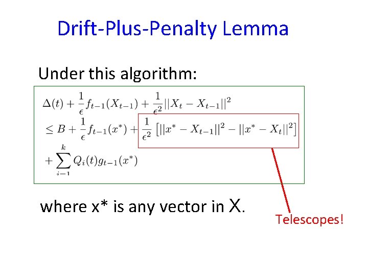
Drift-Plus-Penalty Lemma Under this algorithm: where x* is any vector in X. Telescopes!

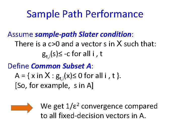
Sample Path Performance Assume sample-path Slater condition: There is a c>0 and a vector s in X such that: gt, i(s)≤ -c for all i , t Define Common Subset A: A = { x in X : gt, i(x)≤ 0 for all i , t }. [So, for example, s in A] We get 1/ε 2 convergence compared to all fixed-decision vectors in A.

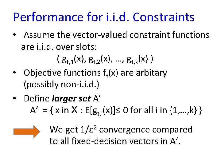
Performance for i. i. d. Constraints • Assume the vector-valued constraint functions are i. i. d. over slots: ( gt, 1(x), gt, 2(x), …, gt, k(x) ) • Objective functions ft(x) are arbitary (possibly non-i. i. d. ) • Define larger set A’ A’ = { x in X : E[gt, i(x)]≤ 0 for all i in {1, …, k} } We get 1/ε 2 convergence compared to all fixed-decision vectors in A’.

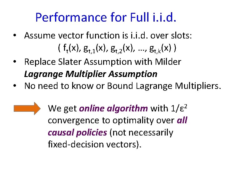
Performance for Full i. i. d. • Assume vector function is i. i. d. over slots: ( ft(x), gt, 1(x), gt, 2(x), …, gt, k(x) ) • Replace Slater Assumption with Milder Lagrange Multiplier Assumption • No need to know or Bound Lagrange Multipliers. We get online algorithm with 1/ε 2 convergence to optimality over all causal policies (not necessarily fixed-decision vectors).

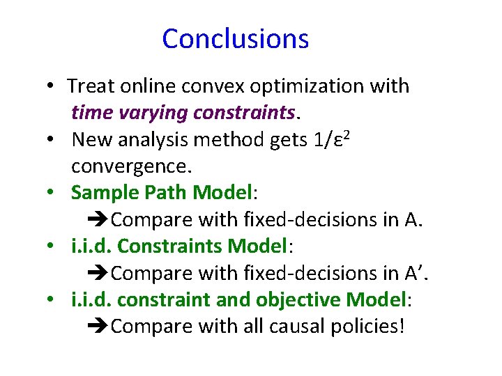
Conclusions • Treat online convex optimization with time varying constraints. • New analysis method gets 1/ε 2 convergence. • Sample Path Model: Compare with fixed-decisions in A. • i. i. d. Constraints Model: Compare with fixed-decisions in A’. • i. i. d. constraint and objective Model: Compare with all causal policies!