OneWay ANOVA Independent Samples Basic Design Grouping variable

One-Way ANOVA Independent Samples

Basic Design • • Grouping variable with 2 or more levels Continuous dependent/criterion variable H : 1 = 2 =. . . = k Assumptions – Homogeneity of variance – Normality in each population

The Model • Yij = + j + eij, or, • Yij - = j + eij. • The difference between the grand mean ( ) and the DV score of subject number i in group number j • is equal to the effect of being in treatment group number j, • plus error, eij

Four Methods of Teaching ANOVA Do these four samples differ enough from each other to reject the null hypothesis that type of instruction has no effect on mean test performance?

Error Variance • Use the sample data to estimate the amount of error variance in the scores. • This assumes that you have equal sample sizes. • For our data, MSE = (. 5 +. 5) / 4 = 0. 5
 =")
Among Groups Variance • • Assumes equal sample sizes VAR(2, 3, 7, 8) = 26 / 3 MSA = 5 26 / 3 = 43. 33 If H is true, this also estimates error variance. • If H is false, this estimates error plus treatment variance.

F • F = MSA / MSE • If H is true, expect F = error/error = 1. • If H is false, expect

Why F ? • Developed by Sir Ronald A. Fisher, who called it the “variance ratio. ” • Renamed “F” by George W. Snedecor, in honor of Fisher.

p • • • F = 43. 33 /. 5 = 86. 66. total df in the k samples is N - 1 = 19 treatment df is k – 1 = 3 error df is k(n - 1) = N - k = 16 Using the F tables in our text book, p <. 01. • One-tailed test of nondirectional hypothesis
2 = (1 - 5)2 + (2")
Deviation Method • SSTOT = (Yij - GM)2 = (1 - 5)2 + (2 - 5)2 +. . . + (9 - 5)2 = 138. • SSA = [nj (Mj - GM)2] • SSA = n (Mj - GM)2 with equal n’s = 5[(2 - 5)2 + (3 - 5)2 + (7 - 5)2 + (8 - 5)2] = 130. • SSE = (Yij - Mj)2 = (1 - 2)2 + (2 - 2)2 +. . + (9 - 8)2 = 8.
 - [(1 +")
Computational Method = (1 + 4 +. . . + 81) - [(1 + 2 +. . . + 9) 2] N = 638 - (100)2 20 = 138. = [102 + 152 + 352 + 402] 5 - (100)2 20 = 130. SSE = SSTOT – SSA = 138 - 130 = 8.

Source Table

Violations of Assumptions • • Check boxplots, histograms, stem & leaf Compare mean to median Compute g 1 (skewness) and g 2 (kurtosis) Kolmogorov-Smirnov Fmax > 4 or 5 ? Screen for outliers Data transformations, nonparametric tests Resampling statistics

Reducing Skewness • Positive – Square root or other root – Log – Reciprocal • Negative – Reflect and then one of the above – Square or other exponent – Inverse log • Trim or Winsorize the samples

Heterogeneity of Variance • Box: True Fcrit is between that for – df = (k-1), k(n-1) and – df = 1, (n-1) – k = 3, n = 10, df = 2, 27 to 1, 9 – F. 05 = 3. 354 to 5. 117 • Welch test • Transformations

Computing ANOVA From Group Means and Variances with Unequal Sample Sizes GM = pj Mj =. 2556(4. 85) +. 2331(4. 61) +. 2707(4. 61) +. 2406(4. 38) = 4. 616. Among Groups SS = 34(4. 85 ‑ 4. 616)2 + 31(4. 61 ‑ 4. 616)2 + 36(4. 61 ‑ 4. 616)2 + 32(4. 38 ‑ 4. 616)2 = 3. 646. With 3 df, MSA = 1. 215, and F(3, 129) = 2. 814, p =. 042.

Heterogeneity of Variance • Look at the SD column. We have this problem. • Box (1954, see our textbook) tells us the critical (. 05) value for our F on this problem is somewhere between F(1, 30) = 4. 17 and F(3, 129) = 2. 675. Unfortunately our F falls in that range, so we don’t know whether or not it is significant.

Welch ANOVA • • • Does not require homogeneity of variance. F and degrees of freedom are adjusted. As with the separate variances t test. See the handout for the computation. SAS will do it for you. F(3, 66) = 3. 910, p =. 012

Directional Hypotheses • • H 1: µ 1 > µ 2 > µ 3 Obtain the usual one-tailed p value Divide it by k! Of course, the predicted ordering must be observed • In this case, a one-sixth tailed test

Fixed, Random, Mixed Effects • A classification variable may be fixed or random • In factorial ANOVA one could be fixed another random • Dose of Drug (random) x Sex of Subject (fixed) • Subjects is a hidden random effects factor.
2 = 137 Group A = 1 B=4 C=3")
ANOVA as Regression SSerror = (Y-Predicted)2 = 137 Group A = 1 B=4 C=3 D=2 Y = a + b. G SSregression = 138 -137=1, r 2 =. 007

Quadratic Regression SSregression = 126, 2 =. 913 Y = a + b 1 G + b 2 G 2

Cubic Regression SSregression = 130, 2 =. 942 Y = a + b 1 G + b 2 G 2 + b 3 G 3

Magnitude of Effect • Omega Square is less biased

Benchmarks for 2 • . 01 is small • . 06 is medium • . 14 is large

Physician’s Aspirin Study • • Small daily dose of aspirin vs. placebo DV = have another heart attack or not Odds Ratio = 1. 83 early in the study Not ethical to continue the research given such a dramatic effect • As a % of variance, the treatment accounted for. 01% of the variance

CI, 2 • Put a confidence interval on eta-squared. • Conf-Interval-R 2 -Regr. sas • If you want the CI to be equivalent to the ANOVA F test you should use a cc of (1 -2 ), not (1 - ). • Otherwise the CI could include zero even though the test is significant.

d versus 2 • I generally prefer d-like statistics over 2 like statistics • If one has a set of focused contrasts, one can simply report d for each. • For the omnibus effect, one can compute the average d across contrasts. • Steiger (2004) has proposed the root mean square standardized effect

Average Contrast d • Orthogonal Contrasts: AB vs BC, A vs B, C vs D. • d = 5. 883, 1. 414. Mean = 2. 90 • A vs BCD, B vs CD, C vs D • d = 1. 922, 5. 565, 1. 414. Mean = 2. 97 • Oops, depends on the particular contasts employed. • SPSS output data

Steiger’s RMSSE • This is an enormous standardized difference between means. • Construct a CI for RMSSE http: //www. statpower. net/Content/NDC. exe
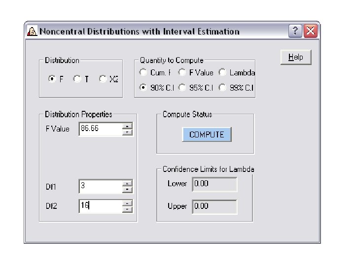
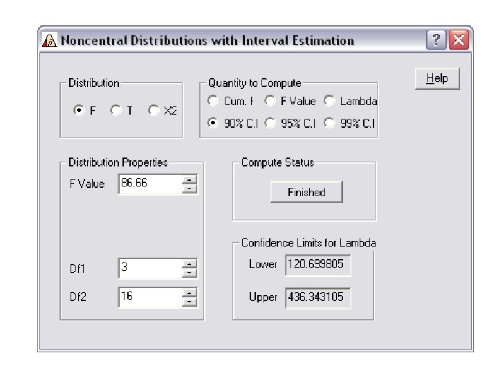

The CI runs from 2. 84 to 5. 39.

Power Analysis • See the handout for doing it by hand. • Better, use a computer to do it. • http: //core. ecu. edu/psyc/wuenschk/docs 30/GPower 3 -ANOVA 1. pdf • The effect size parameter is Cohen’s f • f = the standard deviation of the population means divided by the within-population standard deviation • . 1 = small, . 25 = medium, . 4 = large

APA-Style Presentation
 = 86. 66, MSE")
Teaching method significantly affected the students’ test scores, F(3, 16) = 86. 66, MSE = 0. 50, p <. 001, 2 =. 942, 95% CI [. 858, . 956]. Pairwise comparisons were made with Bonferroni tests, holding familywise error rate at a maximum of. 01. As shown in Table 1, the computer-based and devoted methods produced significantly better student performance than did the ancient and backwards methods.
- Slides: 36