Onestock ELS 1 Introduction s ELS is a

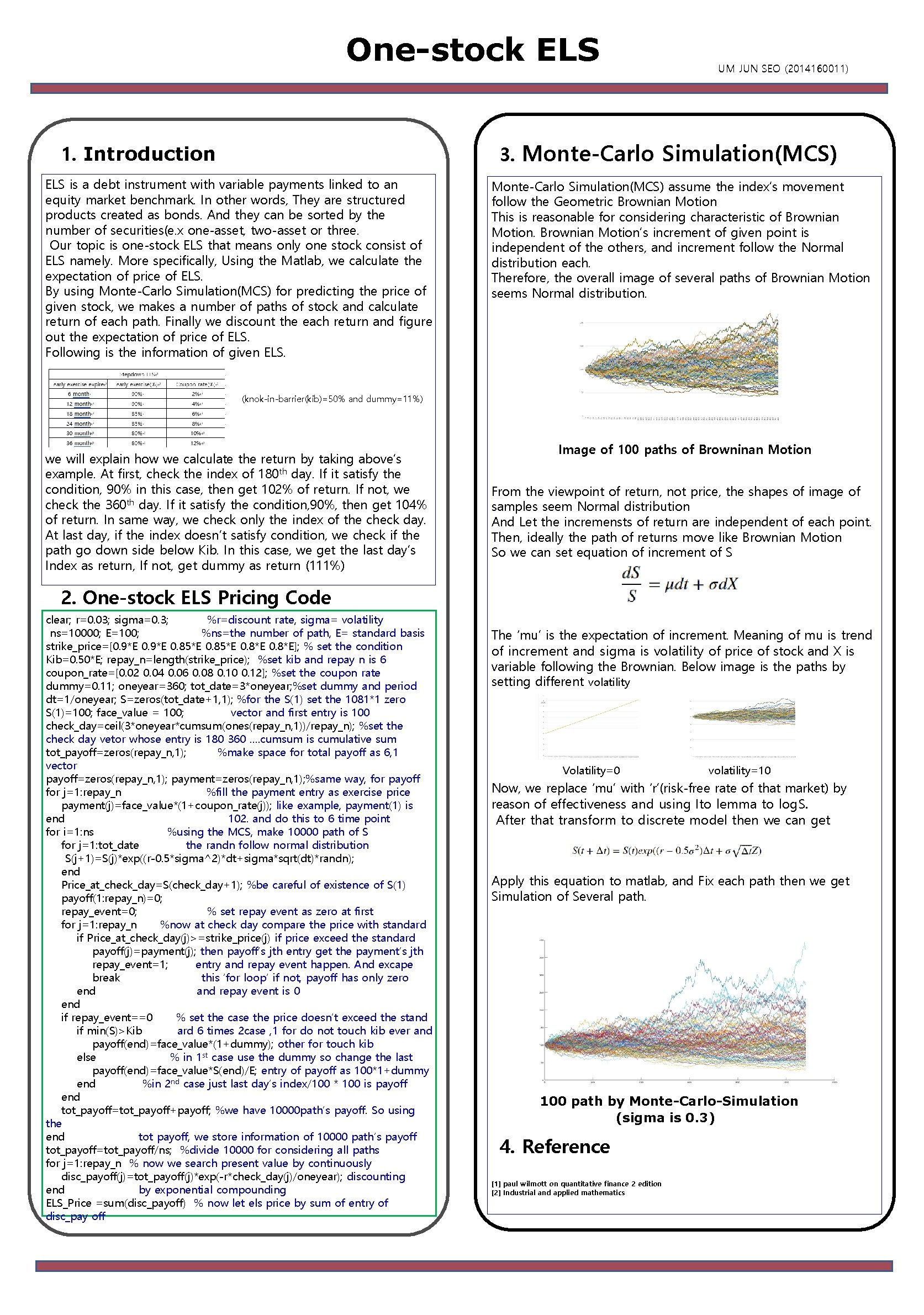
One-stock ELS 1. Introduction s ELS is a debt instrument with variable payments linked to an equity market benchmark. In other words, They are structured products created as bonds. And they can be sorted by the number of securities(e. x one-asset, two-asset or three. Our topic is one-stock ELS that means only one stock consist of ELS namely. More specifically, Using the Matlab, we calculate the expectation of price of ELS. By using Monte-Carlo Simulation(MCS) for predicting the price of given stock, we makes a number of paths of stock and calculate return of each path. Finally we discount the each return and figure out the expectation of price of ELS. Following is the information of given ELS. UM JUN SEO (2014160011) 3. Monte-Carlo Simulation(MCS) assume the index’s movement follow the Geometric Brownian Motion This is reasonable for considering characteristic of Brownian Motion’s increment of given point is independent of the others, and increment follow the Normal distribution each. Therefore, the overall image of several paths of Brownian Motion seems Normal distribution. (knok-in-barrier(kib)=50% and dummy=11%) we will explain how we calculate the return by taking above’s example. At first, check the index of 180 th day. If it satisfy the condition, 90% in this case, then get 102% of return. If not, we check the 360 th day. If it satisfy the condition, 90%, then get 104% of return. In same way, we check only the index of the check day. At last day, if the index doesn’t satisfy condition, we check if the path go down side below Kib. In this case, we get the last day’s Index as return, If not, get dummy as return (111%) Image of 100 paths of Browninan Motion From the viewpoint of return, not price, the shapes of image of samples seem Normal distribution And Let the incremensts of return are independent of each point. Then, ideally the path of returns move like Brownian Motion So we can set equation of increment of S 2. One-stock ELS Pricing Code clear; r=0. 03; sigma=0. 3; %r=discount rate, sigma= volatility ns=10000; E=100; %ns=the number of path, E= standard basis strike_price=[0. 9*E 0. 85*E 0. 8*E]; % set the condition Kib=0. 50*E; repay_n=length(strike_price); %set kib and repay n is 6 coupon_rate=[0. 02 0. 04 0. 06 0. 08 0. 10 0. 12]; %set the coupon rate dummy=0. 11; oneyear=360; tot_date=3*oneyear; %set dummy and period dt=1/oneyear; S=zeros(tot_date+1, 1); %for the S(1) set the 1081*1 zero S(1)=100; face_value = 100; vector and first entry is 100 check_day=ceil(3*oneyear*cumsum(ones(repay_n, 1))/repay_n); %set the check day vetor whose entry is 180 360 …. cumsum is cumulative sum tot_payoff=zeros(repay_n, 1); %make space for total payoff as 6, 1 vector payoff=zeros(repay_n, 1); payment=zeros(repay_n, 1); %same way, for payoff for j=1: repay_n %fill the payment entry as exercise price payment(j)=face_value*(1+coupon_rate(j)); like example, payment(1) is end 102. and do this to 6 time point for i=1: ns %using the MCS, make 10000 path of S for j=1: tot_date the randn follow normal distribution S(j+1)=S(j)*exp((r-0. 5*sigma^2)*dt+sigma*sqrt(dt)*randn); end Price_at_check_day=S(check_day+1); %be careful of existence of S(1) payoff(1: repay_n)=0; repay_event=0; % set repay event as zero at first for j=1: repay_n %now at check day compare the price with standard if Price_at_check_day(j)>=strike_price(j) if price exceed the standard payoff(j)=payment(j); then payoff’s jth entry get the payment’s jth repay_event=1; entry and repay event happen. And excape break this ‘for loop’ if not, payoff has only zero end and repay event is 0 end if repay_event==0 % set the case the price doesn’t exceed the stand if min(S)>Kib ard 6 times 2 case , 1 for do not touch kib ever and payoff(end)=face_value*(1+dummy); other for touch kib else % in 1 st case use the dummy so change the last payoff(end)=face_value*S(end)/E; entry of payoff as 100*1+dummy end %in 2 nd case just last day’s index/100 * 100 is payoff end tot_payoff=tot_payoff+payoff; %we have 10000 path’s payoff. So using the end tot payoff, we store information of 10000 path’s payoff tot_payoff=tot_payoff/ns; %divide 10000 for considering all paths for j=1: repay_n % now we search present value by continuously disc_payoff(j)=tot_payoff(j)*exp(-r*check_day(j)/oneyear); discounting end by exponential compounding ELS_Price =sum(disc_payoff) % now let els price by sum of entry of disc_pay off The ‘mu’ is the expectation of increment. Meaning of mu is trend of increment and sigma is volatility of price of stock and X is variable following the Brownian. Below image is the paths by paul wilmott on quantitative finance setting different volatility Volatility=0 volatility=10 Now, we replace ‘mu’ with ‘r’(risk-free rate of that market) by reason of effectiveness and using Ito lemma to log. S. After that transform to discrete model then we can get Apply this equation to matlab, and Fix each path then we get Simulation of Several path. 100 path by Monte-Carlo-Simulation (sigma is 0. 3) 4. Reference [1] paul wilmott on quantitative finance 2 edition [2] Industrial and applied mathematics