One more PCA Example Generalized linear models Poisson

One more PCA Example Generalized linear models – Poisson distribution Generalized linear models – Negative binomial distribution Generalized linear models – logistic regression (binomial distribution)

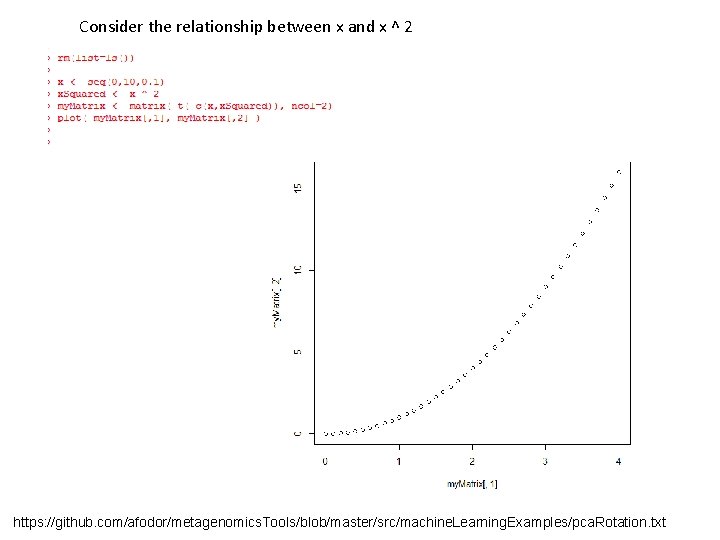
Consider the relationship between x and x ^ 2 https: //github. com/afodor/metagenomics. Tools/blob/master/src/machine. Learning. Examples/pca. Rotation. txt

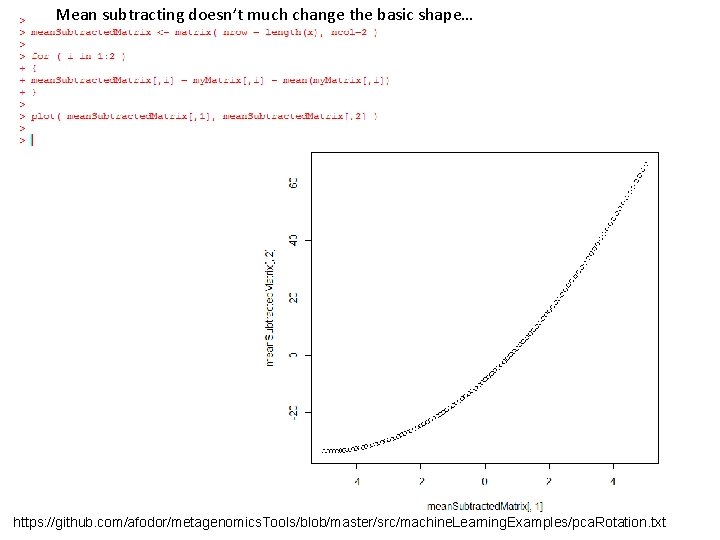
Mean subtracting doesn’t much change the basic shape… https: //github. com/afodor/metagenomics. Tools/blob/master/src/machine. Learning. Examples/pca. Rotation. txt

We can perform the PCA via Eigen value rotation [200, 2] * [2, 2] = [200, 2] https: //github. com/afodor/metagenomics. Tools/blob/master/src/machine. Learning. Examples/pca. Rotation. txt

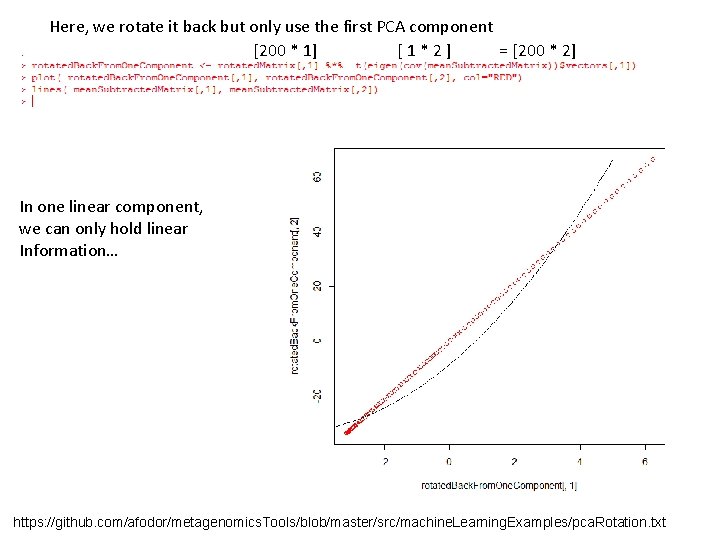
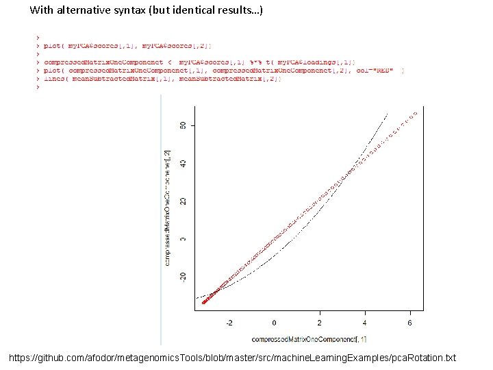
Here, we rotate it back but only use the first PCA component [200 * 1] [1*2] = [200 * 2] In one linear component, we can only hold linear Information… https: //github. com/afodor/metagenomics. Tools/blob/master/src/machine. Learning. Examples/pca. Rotation. txt

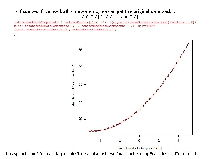
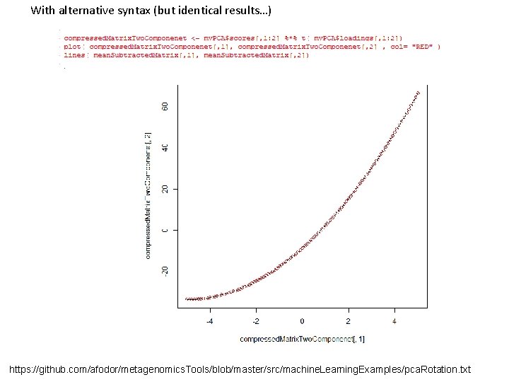
Of course, if we use both components, we can get the original data back… [200 * 2] * [2, 2] = [200 * 2] https: //github. com/afodor/metagenomics. Tools/blob/master/src/machine. Learning. Examples/pca. Rotation. txt

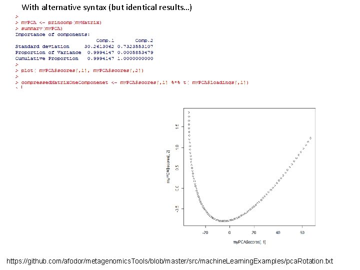
With alternative syntax (but identical results…) https: //github. com/afodor/metagenomics. Tools/blob/master/src/machine. Learning. Examples/pca. Rotation. txt

With alternative syntax (but identical results…) https: //github. com/afodor/metagenomics. Tools/blob/master/src/machine. Learning. Examples/pca. Rotation. txt

With alternative syntax (but identical results…) https: //github. com/afodor/metagenomics. Tools/blob/master/src/machine. Learning. Examples/pca. Rotation. txt

One more PCA Example Generalized linear models – Poisson distribution Generalized linear models – Negative binomial distribution Generalized linear models – logistic regression (binomial distribution)

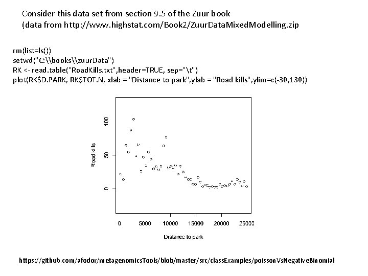
Consider this data set from section 9. 5 of the Zuur book (data from http: //www. highstat. com/Book 2/Zuur. Data. Mixed. Modelling. zip rm(list=ls()) setwd("C: \books\zuur. Data") RK <- read. table("Road. Kills. txt", header=TRUE, sep="t") plot(RK$D. PARK, RK$TOT. N, xlab = "Distance to park", ylab = "Road kills", ylim=c(-30, 130)) https: //github. com/afodor/metagenomics. Tools/blob/master/src/class. Examples/poisson. Vs. Negative. Binomial

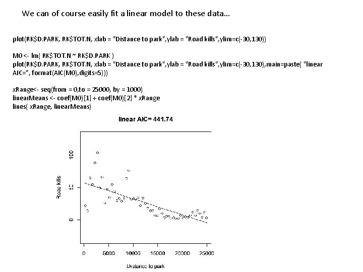
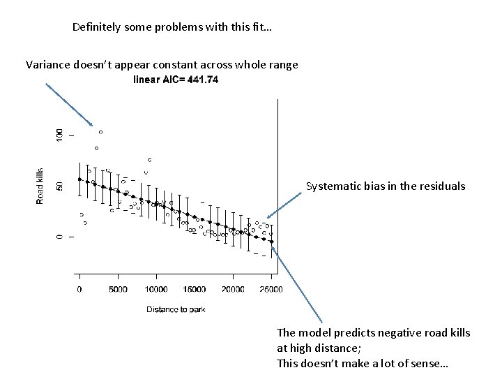
We can of course easily fit a linear model to these data… plot(RK$D. PARK, RK$TOT. N, xlab = "Distance to park", ylab = "Road kills", ylim=c(-30, 130)) M 0 <- lm( RK$TOT. N ~ RK$D. PARK ) plot(RK$D. PARK, RK$TOT. N, xlab = "Distance to park", ylab = "Road kills", ylim=c(-30, 130), main=paste( "linear AIC=", format(AIC(M 0), digits=5))) x. Range<- seq(from = 0, to = 25000, by = 1000) linear. Means <- coef(M 0)[1] + coef(M 0)[2] * x. Range lines( x. Range, linear. Means)

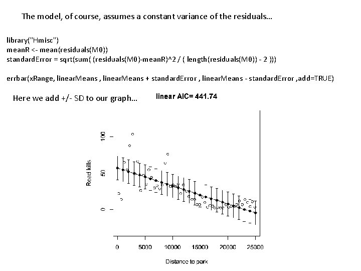
The model, of course, assumes a constant variance of the residuals… library("Hmisc") mean. R <- mean(residuals(M 0)) standard. Error = sqrt(sum( (residuals(M 0)-mean. R)^2 / ( length(residuals(M 0)) - 2 ))) errbar(x. Range, linear. Means + standard. Error , linear. Means - standard. Error , add=TRUE) Here we add +/- SD to our graph…

Definitely some problems with this fit… Variance doesn’t appear constant across whole range Systematic bias in the residuals The model predicts negative road kills at high distance; This doesn’t make a lot of sense…

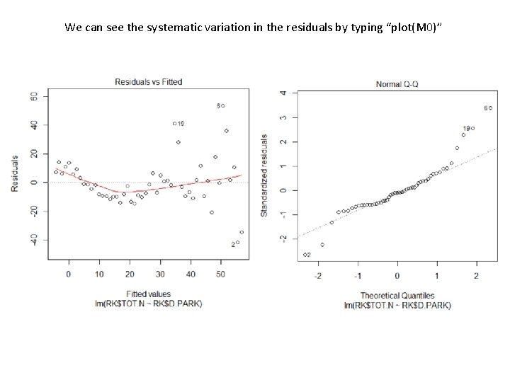
We can see the systematic variation in the residuals by typing “plot(M 0)”

It would be nice if we could have a model based on counts that allows us to vary the variance ; We will see that we can build a model based on the negative binomial distribution that fits the bill. But let’s first (for simplicity) consider a model based on the Poisson distribution.

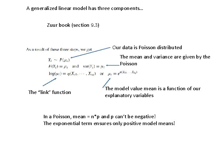
A generalized linear model has three components… Zuur book (section 9. 3) Our data is Poisson distributed The mean and variance are given by the Poisson The “link” function The model value mean is a function of our explanatory variables In a Poisson, mean = n*p and p can’t be negative! The exponential term ensures only positive model means!

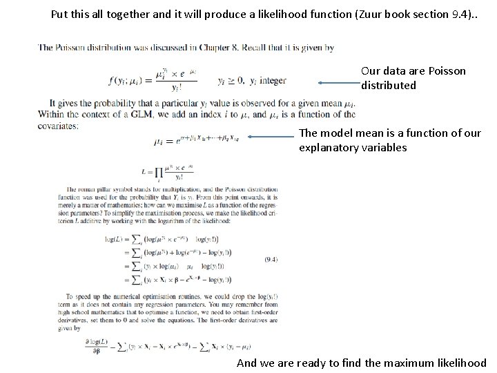
Put this all together and it will produce a likelihood function (Zuur book section 9. 4). . Our data are Poisson distributed The model mean is a function of our explanatory variables And we are ready to find the maximum likelihood

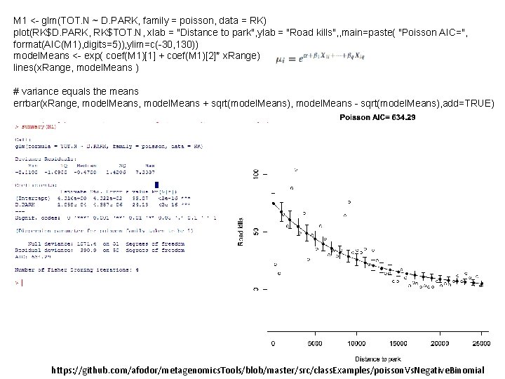
M 1 <- glm(TOT. N ~ D. PARK, family = poisson, data = RK) plot(RK$D. PARK, RK$TOT. N, xlab = "Distance to park", ylab = "Road kills", , main=paste( "Poisson AIC=", format(AIC(M 1), digits=5)), ylim=c(-30, 130)) model. Means <- exp( coef(M 1)[1] + coef(M 1)[2]* x. Range) lines(x. Range, model. Means ) # variance equals the means errbar(x. Range, model. Means + sqrt(model. Means), model. Means - sqrt(model. Means), add=TRUE) https: //github. com/afodor/metagenomics. Tools/blob/master/src/class. Examples/poisson. Vs. Negative. Binomial

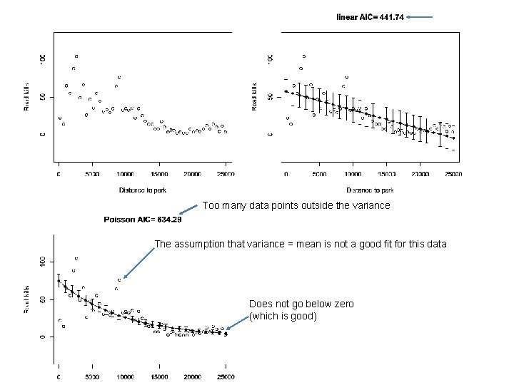
Too many data points outside the variance The assumption that variance = mean is not a good fit for this data Does not go below zero (which is good)

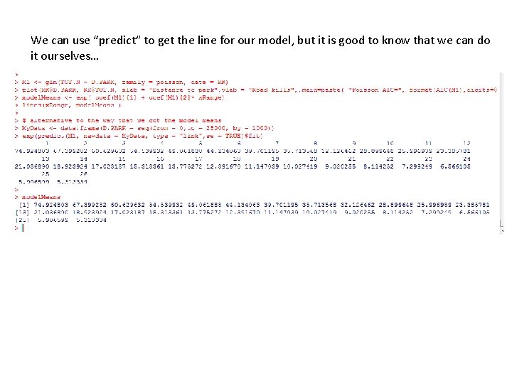
We can use “predict” to get the line for our model, but it is good to know that we can do it ourselves…

One more PCA Example Generalized linear models – Poisson distribution Generalized linear models – Negative binomial distribution Generalized linear models – logistic regression (binomial distribution)

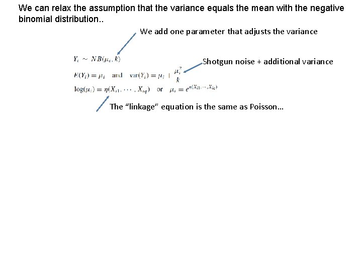
We can relax the assumption that the variance equals the mean with the negative binomial distribution. . We add one parameter that adjusts the variance Shotgun noise + additional variance The “linkage” equation is the same as Poisson…

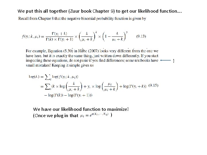
We put this all together (Zuur book Chapter 9) to get our likelihood function…. ! We have our likelihood function to maximize! ) (Once we plug in that

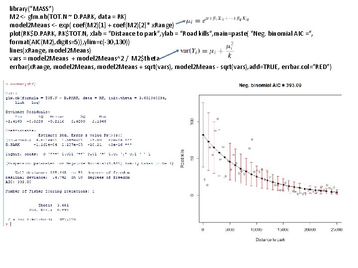
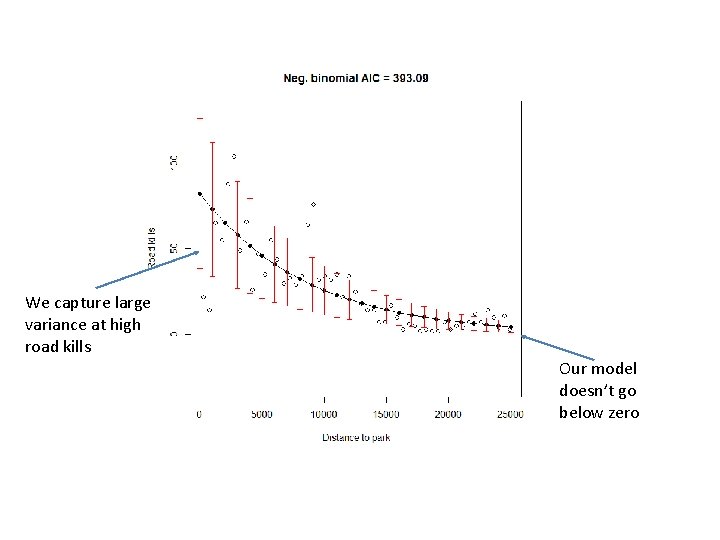
library("MASS") M 2 <- glm. nb(TOT. N ~ D. PARK, data = RK) model 2 Means <- exp( coef(M 2)[1] + coef(M 2)[2]* x. Range) plot(RK$D. PARK, RK$TOT. N, xlab = "Distance to park", ylab = "Road kills", main=paste( "Neg. binomial AIC =", format(AIC(M 2), digits=5)), ylim=c(-30, 130)) lines(x. Range, model 2 Means) vars = model 2 Means + model 2 Means^2 / M 2$theta errbar(x. Range, model 2 Means + sqrt(vars), model 2 Means - sqrt(vars), add=TRUE, errbar. col="RED")

We capture large variance at high road kills Our model doesn’t go below zero

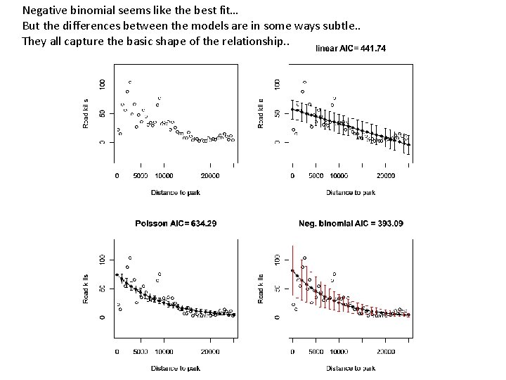
Negative binomial seems like the best fit… But the differences between the models are in some ways subtle. . They all capture the basic shape of the relationship. .

One more PCA Example Generalized linear models – Poisson distribution Generalized linear models – Negative binomial distribution Generalized linear models – logistic regression (binomial distribution)

What about binary variables. voting democratic or republican has cancer/does not have cancer

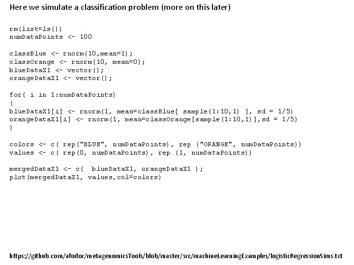
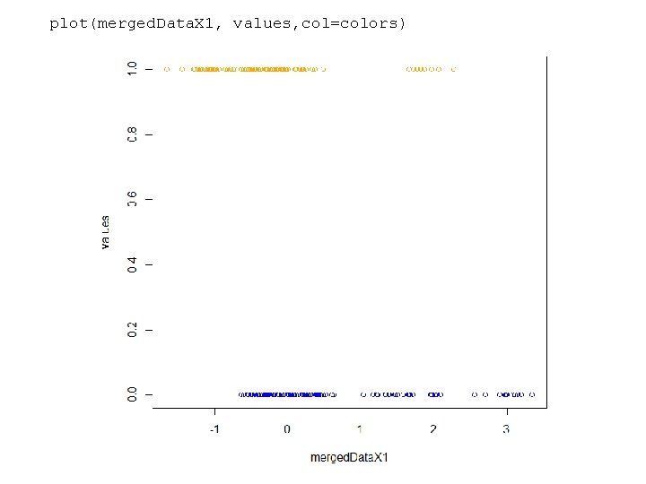
Here we simulate a classification problem (more on this later) rm(list=ls()) num. Data. Points <- 100 class. Blue <- rnorm(10, mean=1); class. Orange <- rnorm(10, mean=0); blue. Data. X 1 <- vector(); orange. Data. X 1 <- vector(); for( i in 1: num. Data. Points) { blue. Data. X 1[i] <- rnorm(1, mean=class. Blue[ sample(1: 10, 1) ], sd = 1/5) orange. Data. X 1[i] <- rnorm(1, mean=class. Orange[sample(1: 10, 1)], sd = 1/5) } colors <- c( rep("BLUE", num. Data. Points), rep ("ORANGE", num. Data. Points)) values <- c( rep(0, num. Data. Points), rep (1, num. Data. Points)) merged. Data. X 1 <- c( blue. Data. X 1, orange. Data. X 1 ); plot(merged. Data. X 1, values, col=colors) https: //github. com/afodor/metagenomics. Tools/blob/master/src/machine. Learning. Examples/logistic. Regression. Sims. txt

plot(merged. Data. X 1, values, col=colors)

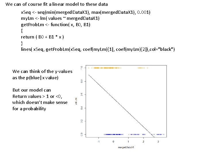
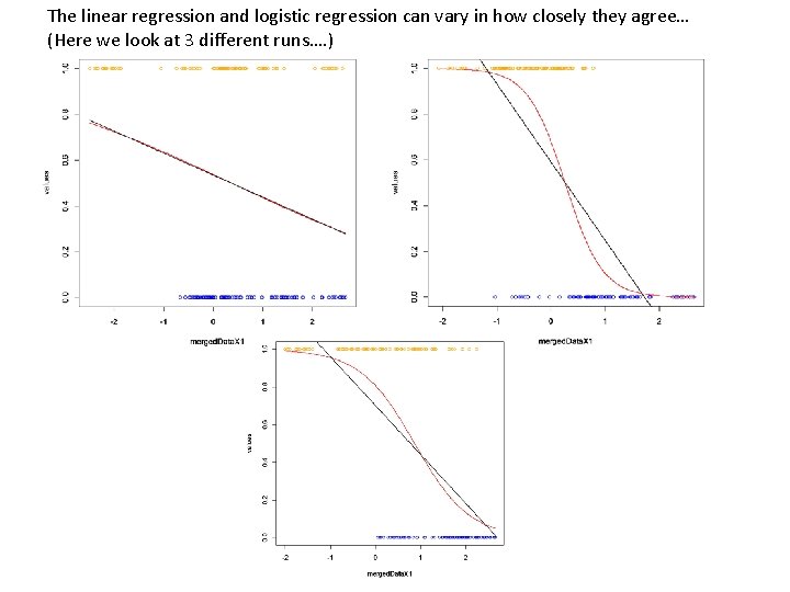
We can of course fit a linear model to these data x. Seq <- seq(min(merged. Data. X 1), max(merged. Data. X 1), 0. 001) my. Lm <- lm( values ~ merged. Data. X 1) get. Prob. Lm <- function( x, B 0, B 1) { return ( B 0 + B 1 * x ) } lines( x. Seq, get. Prob. Lm(x. Seq, coef(my. Lm)[1], coef(my. Lm)[2]), col="black") We can think of the y-values as the p(blue|x value) But our model can Return values > 1 or <0, which doesn’t make sense for a probability

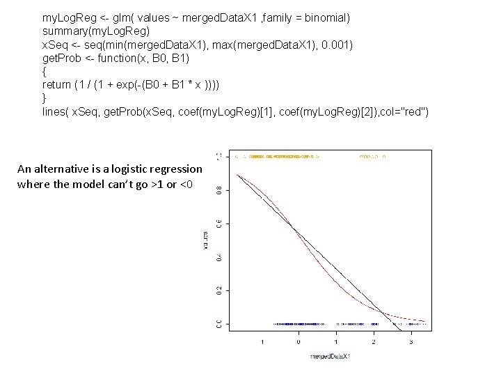
my. Log. Reg <- glm( values ~ merged. Data. X 1 , family = binomial) summary(my. Log. Reg) x. Seq <- seq(min(merged. Data. X 1), max(merged. Data. X 1), 0. 001) get. Prob <- function(x, B 0, B 1) { return (1 / (1 + exp(-(B 0 + B 1 * x )))) } lines( x. Seq, get. Prob(x. Seq, coef(my. Log. Reg)[1], coef(my. Log. Reg)[2]), col="red") An alternative is a logistic regression where the model can’t go >1 or <0

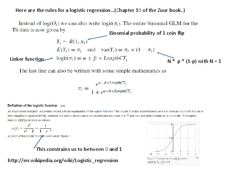
Here are the rules for a logistic regression…(Chapter 10 of the Zuur book. . ) Binomial probability of 1 coin flip Linker function This constrains us to between 0 and 1 http: //en. wikipedia. org/wiki/Logistic_regression N * p * (1 -p) with N = 1

Put all this together into the likelihood… Binomial distribution with n = 1 Yi is 1 or 0 This is if a head (1 - ) if a tail Find the parameters to maximize this and we are good to go…. http: //www. stat. cmu. edu/~cshalizi/u. ADA/12/lectures/ch 12. pdf

The linear regression and logistic regression can vary in how closely they agree… (Here we look at 3 different runs…. )

Next: Zero inflated Poisson and Negative Binomial