ONE DAY WORKSHOP ON BASIC RESEARCH METHODOLOGY 17

ONE DAY WORKSHOP ON BASIC RESEARCH METHODOLOGY 17 th December 2016 Prof. Prakash Kumar Retd. Jr. Scientist-cum-Asst. Prof. Dept. of Agril. Statistics Birsa Agricultural University, Ranchi

Objective of the Workshop Participants are expected to: – Understand the basic notion of statistics in research – Learn various statistical techniques used to analyze data – Be able to interpret results and draw conclusion – Learn the tools used in the analysis of data

Research Design and Methodology • Research is the process of investigating scientific questions • Steps in Research process– Defining the problem and conceptualizing the study – Designing and conducting study • Collecting data • Analyzing data – Making sense of data

Statistics is science of data collection, summarization, analysis and interpretation.

DATA COLLECTION Statistical Data can be Primary or Secondary. Primary data are those which are collected for the first time either by conducting survey or experiment and thus original in character. Whereas secondary data are those which have already been collected by some other persons and which have passed through the statistical process at least once.

SUMMARISATION OF DATA When data are collected by any survey or experiments, those primary data are in the shape of raw materials to which statistical methods are to be applied for the analysis and interpretation. The data contained in schedules and questionnaires are not directly fit for analysis and interpretation. So it is essential that those data are made available in condensed form for further treatment. For this purpose data are divided and classified in homogeneous groups and then tabulated as per needs. Types of classifications : 1. Geographical 2. Chronological 3. Qualitative 4. Quantitative Types of Tabulations: 1. Simple and Complex Tabulation a. One way table b. Two way table c. Three way table d. Higher Order table 2. General and Special Purposes table

A Taxonomy of Statistics

How does statistics help us? Ages (in month) of the 60 patients in our data set 1 are- 71, 127, 65, 82, 140, 53, 114, 56, 84, 65, 67, 134, 64, …. , 91, 51 By simply looking at the data, we fail to produce any informative account to describe the data, how ever, statistics produce a quick insight in to data using graphical Mean 90. 41666667 and numerical statistical tools Standard Error 3. 902649518 Median 84 Mode 84 Standard Deviation 30. 22979318 Sample Variance 913. 8403955 Kurtosis Skewness -1. 183899591 0. 389872725 Range 95 Minimum 48 Maximum 143 Sum Count 5425 60

Statistical Description of Data • Statistics describes a numeric set of data by its • Center (mean, median, mode etc) • Variability (standard deviation, range etc) • Shape (skewness, kurtosis etc) • Statistics describes a categorical set of data by • Frequency, percentage or proportion of each category

Statistical Inference Sample Population • Statistical inference is the process by which we acquire information about populations from samples.

Parameter vs Statistics • Parameter: – Any statistical characteristic of a population. – Population mean, population median, population standard deviation are examples of parameters. – Parameter describes the distribution of a population – Parameters are fixed and usually unknown

Parameter vs Statistics • Statistic: Any statistical characteristic of a sample. – Sample mean, sample median, sample standard deviation are some examples of statistics. – Statistic describes the distribution of population – Value of a statistic is known and is varies for different samples – Are used for making inference on parameter

Parameter vs Statistics • Statistical Issue: To describe the distribution of a population through census or making inference on population distribution/ population parameter using sample distribution/ statistic. • E. g. sample mean is an estimate of the population mean

Variable - any characteristic of an individual or entity. A variable can take different values for different individuals. Distribution - (of a variable) tells us what values the variable takes and how often it takes these values. • Unimodal - having a single peak • Bimodal - having two distinct peaks • Symmetric - left and right half are mirror images.

FREQUENCY DISTRIBUTION

DIAGRAMATIC PRESENTATION OF DATA Graphical Presentation: We look for the overall pattern and for striking deviations from that pattern. Over all pattern usually described by shape, center, and spread of the data. An individual value that falls outside the overall pattern is called an outlier. Bar diagram , Pie charts , Histogram, stem and leaf and Box-plot etc are used variables.

Descriptive Statistics After collecting data we go for its classifications, tabulations and also for its graphical or diagrammatical presentation. These measures help in reducing the size of the data and enable us to make some comparative studies of related variables But these derivatives are not enough. Hence we further wish to reduce the complexicity of data and to make them comparable. For this we apply various statistical tools available such as Measures of Central Tendencies, Measures of dispersion etc.

MEASURESS OF CENTRAL TENDEENCIES

MEAN, MEDIAN AND MODE

MEASURES OF DISPERSION The mean, median and mode are measures of central tendencies of a variable, but they do not provide any information of how much the measurements vary or are spread. . Measures of dispersion or variation are another statistical tool to estimate the homogeneity or heterogeneity in the data set. There are different measures of dispersion such as Range, Mean Deviation, Standard Deviation, Variance and Standard Error. Whereas another measure of dispersion i. e. Coefficient of Variation( expressed in %) is also available which is a relative measure of dispersion.

Range : Mean Deviation:

Standard Deviation:

Variance : Variance = (S. D. )2 Standard Error : It is given by S. E. = S. D. / √n Coefficient of Variation (%) : C. V. (%) = S. E. * 100/ Grand Mean

Hypothesis Testing/ Test of Significance :

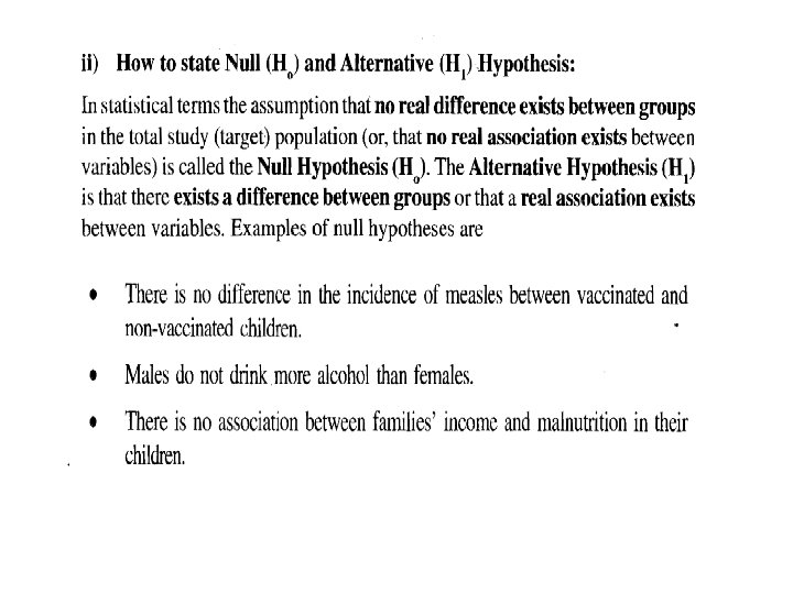
Hypothesis : Hypothesis means a statement. It can be of two types : Statistical Hypothesis and Non statistical hypothesis. In Statistical Hypothesis, some statistical parameters such as mean or variance are involved whereas in non statistical hypothesis no statistical parameters are involved. Null Hypothesis is represented by H 0 whereas alternate hypothesis is represented by H 1. Example of statistical hypothesis is H 0 : µ 1= µ 2 H 1: µ 1 ≠ µ 2 Example of non statistical hypothesis is H 0: The defendant is innocent. H 1: The defendant is guilty.

Null Hypothesis vs. Alternative Hypothesis Null Hypothesis Alternative Hypothesis • Statement about the value of a population parameter • Represented by H 0 • Always stated as an Equality • Statement about the value of a population parameter that must be true if the null hypothesis is false • Represented by H 1 • Stated in on of three forms • > • < •

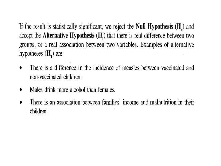
Steps in hypothesis • Hypothesis testing steps: – 1. Null (Ho) and alternative (H 1)hypothesis specification – 2. Selection of significance level (alpha) - 0. 05 or 0. 01 – 3. Calculating the test statistic –e. g. t, F, Chi-square – 4. Calculating the probability value (p-value) or confidence Interval? – 5. Describing the result and statistic in an understandable way.

Type I and Type II Error

Paired and Unpaired Tests:

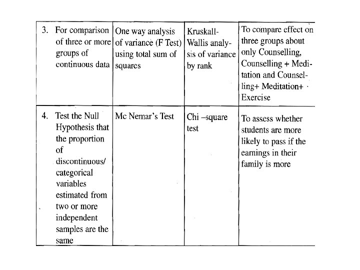
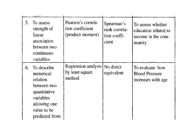
Selection of appropriate Tests :

t-test

Paired t-test

Z -test

VARIANCE RATIO TEST i. e. F - TEST

CHI SQUARE TEST The chi square distribution is a theoretical or mathematical distribution which has wide applicability in statistical work. The term `chi square' (pronounced with a hard `ch') is used because the Greek letter X 2 is used to define this distribution. It will be seen that the elements on which this distribution is based are squared, so that the symbol 2 is used to denote the distribution. For both the goodness of fit test and the test of independence, the chi square statistic is the same. For both of these tests, all the categories into which the data have been divided are used. The data obtained from the sample are referred to as the observed numbers of cases. These are the frequencies of occurrence for each category into which the data have been grouped. In the chi square tests, the null hypothesis makes a statement concerning how many cases are to be expected in each category if this hypothesis is correct. The chi square test is based on the difference between the observed and the expected values for each category. The chi square statistic is defined as where Oi is the observed number of cases in category i, and Ei is the expected number of cases in category i.

CORRELATION

REGRESSION

Introduction to Experimental design The study of strategies for efficient plans for the collection of data, which lead to proper estimates of parameters relevant to the researcher’s objective, is known as experimental design. A properly designed experiment, for a particular research objective, is the basis of all successful experiments. There are three basic principles of experimental design. These are 1. Replication 2. Randomization 3. Control

Terminology of experimental design 1. An experiment is a planned inquiry to obtain new knowledge or to confirm or deny previous results. 2. The population of inference is the set of ALL entities to which the researcher intends to have the results of the experiment be applicable. 3. The experimental unit is the smallest entity to which the treatment is applied and which is capable of being assigned a different treatment independently of other experimental units if the randomization was repeated. This is the most seriously misunderstood and incorrectly applied aspect of experimental design. 4. A factor is a procedure or condition whose effect is to be measured.

5. A level of a factor is a specific manifestation of the factor to be included in the experiment. 6. Experimental error is a measure of the variation which exists among experimental units treated alike. 7. A factor level is said to be replicated if it occurs in more than one experimental unit in the experiment. 8. Randomization in the application of factor levels to experimental units occurs only if each experimental unit has equal and independent chance of receiving any factor level and if each experimental unit is subsequently handled independently.

Replication Although randomization helps to insure that treatment groups are as similar as possible, the results of a single experiment, applied to a small number of objects or subjects, should not be accepted without question. To improve the significance of an experimental result, replication, the repetition of an experiment on a large group of treatments, is required. Replication reduces variability in experimental results, increasing their significance and the confidence level with which a researcher can draw conclusions about an experimental factor.

Randomization involves randomly allocating the experimental units across the treatment groups. Thus, if the experiment compares new maize varieties against a check variety, which is used as a control, then new varieties are allocated to the plots, or experimental units, randomly. In the design of experiments, varieties are allocated to the experimental units not experimental units to the varieties. In experimental design we consider the treatments, or varieties, as data values or levels of a factor (or combination of factors) that are in our controlled study. Randomization is the process by which experimental units (the basic objects upon which the study or experiment is carried out) are allocated to treatments; that is, by a random process and not by any subjective and hence possibly biased approach. The treatments or varieties should be allocated to units in such a way that each treatment is equally likely to be applied to each unit. Because it is generally extremely difficult for experimenters to eliminate bias using only their expert judgment, the use of randomization in experiments is common practice. In a randomized experimental design, objects or individuals are randomly assigned (by chance) to an experimental group. Use of randomization is the most reliable method of creating homogeneous treatment groups, without involving any potential biases or judgments.

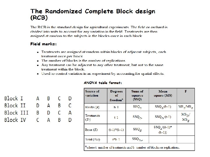
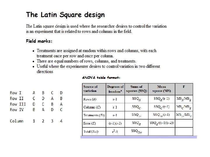
Control of local variability – blocking In the design of experiments, blocking is the arrangement of experimental units into groups(blocks) that are similar to one another. For example, if an experiment is designed to test 36 new maize varieties, the field in which the varieties are to be tested may not be uniform, having two fertility gradients – low and high soil fertility. The level of fertility may introduce a level of variability within the experiment; therefore, blocking is required to remove the effect of low and high fertility. This reduces sources of variability and thus leads to greater precision. For randomized block designs, one factor or variable is of primary interest. However, there also several other nuisance factors. Blocking is used to reduce or eliminate the contribution of nuisance factors to experimental error. The basic concept is to create homogeneous blocks in which the nuisance factors are held constant while the factor of interest is allowed to vary. Within blocks, it is possible to assess the effect of different levels of the factor of interest without having to worry about variations due to changes of the block factors, which are accounted for in the analysis.

The Completely Randomized Design (CRD) The CRD is the simplest of all designs. It is equivalent to a t-test when only two treatments are examined. Field marks: • Replications of treatments are assigned completely at random to independent experimental subjects. • Adjacent subjects could potentially have the same treatment. A 1 D 1 B 2 C 4 B 1 A 3 D 3 A 4 C 1 D 2 C 3 B 4 A 2 C 2 B 3 D 4

Brief concept of Statistical Software • There are many software packages to perform statistical analysis and visualization of data. Some of them are– System for Statistical Analysis (SAS), S-plus, R, Matlab, Minitab, BMDP, STATA, SPSS, Stat. Xact, Statistica, LISREL, JMP, GLIM, HIL, MS Excel etc. , Indo. Stat, Kyplot etc.

Microsoft Excel A Spreadsheet Application. It features calculation, graphing tools, pivot tables and a macro programming language called VBA (Visual Basic for Applications). There are many versions of MS-Excel XP, Excel 2003, Excel 2007 are capable of performing a number of statistical analyses. Starting MS Excel: Double click on the Microsoft Excel icon on the desktop or Click on Start --> Programs --> Microsoft Excel. Worksheet: Consists of a multiple grid of cells with numbered rows down the page and alphabetically-tilted columns across the page. Each cell is referenced by its coordinates. For example, A 3 is used to refer to the cell in column A and row 3. B 10: B 20 is used to refer to the range of cells in column B and rows 10 through 20.

Microsoft Excel Opening a document: File Open (From a existing workbook). Change the directory area or drive to look for file in other locations. Creating a new workbook: File New Blank Document Saving a File: File Save Selecting more than one cell: Click on a cell e. g. A 1), then hold the Shift key and click on another (e. g. D 4) to select cells between and A 1 and D 4 or Click on a cell and drag the mouse across the desired range. Creating Formulas: 1. Click the cell that you want to enter the formula, 2. Type = (an equal sign), 3. Click the Function Button, 4. Select the formula you want and step through the on-screen instructions.

Microsoft Excel Entering Date and Time: Dates are stored as MM/DD/YYYY. No need to enter in that format. For example, Excel will recognize Jan 9 or jan-9 as 1/9/2007 and Jan 9, 1999 as 1/9/1999. To enter today’s date, press Ctrl and ; together. Use a or p to indicate am or pm. For example, 8: 30 p is interpreted as 8: 30 pm. To enter current time, press Ctrl and : together. Copy and Paste all cells in a Sheet: Ctrl+A for selecting, Ctrl +C for copying and Ctrl+V for Pasting. Sorting: Data Sort By … Descriptive Statistics and other Statistical methods: Tools Data Analysis Statistical method. If Data Analysis is not available then click on Tools Add-Ins and then select Analysis Tool. Pack and Analysis tool. Pack-Vba

Microsoft Excel Statistical and Mathematical Function: Start with ‘=‘ sign and then select function from function wizard Inserting a Chart: Click on Chart Wizard (or Insert Chart), select chart, give, Input data range, Update the Chart options, and Select output range/ Worksheet. Importing Data in Excel: File open File. Type Click on File Choose Option ( Delimited/Fixed Width) Choose Options (Tab/ Semicolon/ Comma/ Space/ Other) Finish. Limitations: Excel uses algorithms that are vulnerable to rounding and truncation errors and may produce inaccurate results in extreme cases.

Thank You.