On using global optimization for approximating hull solution

On using global optimization for approximating hull solution of parametric interval systems Iwona Skalna AGH University of Science & Technology, Poland Andrzej Pownuk The University of Texas, El Paso, USA 3 RD NSF Workshop on Imprecise Probability in Engineering Analysis & Design February 20 -22, 2008 | Georgia Institute of Technology, Savannah, USA

Outline ¥ Parametric interval linear systems ¥ Global optimization Monotonicity test Subdivision directions Multidivision ¥ Examples ¥ Concluding remarks acceleration techniques 3 RD NSF Workshop on Imprecise Probability in Engineering Analysis & Design February 20 -22, 2008 | Georgia Institute of Technology, Savannah, USA 2

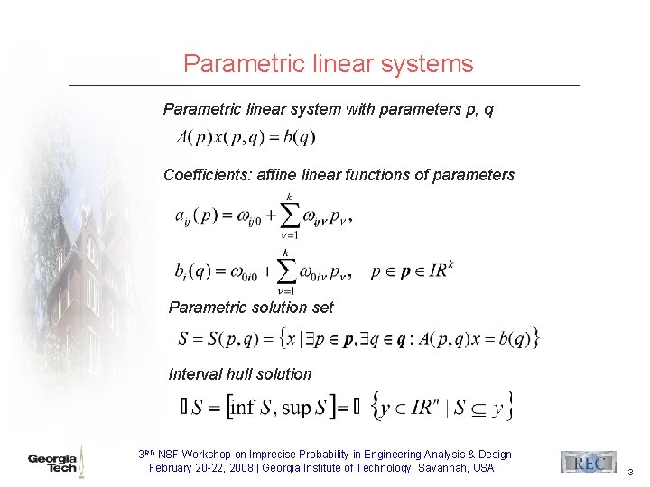
Parametric linear systems Parametric linear system with parameters p, q Coefficients: affine linear functions of parameters Parametric solution set Interval hull solution 3 RD NSF Workshop on Imprecise Probability in Engineering Analysis & Design February 20 -22, 2008 | Georgia Institute of Technology, Savannah, USA 3

Optimization problem (hull solution) Theorem Let A(p) be regular, p IRk, and ximin, ximax denote the global solutions of the i-th minimization and, respectively, maximization problem Then the interval vector 3 RD NSF Workshop on Imprecise Probability in Engineering Analysis & Design February 20 -22, 2008 | Georgia Institute of Technology, Savannah, USA 4

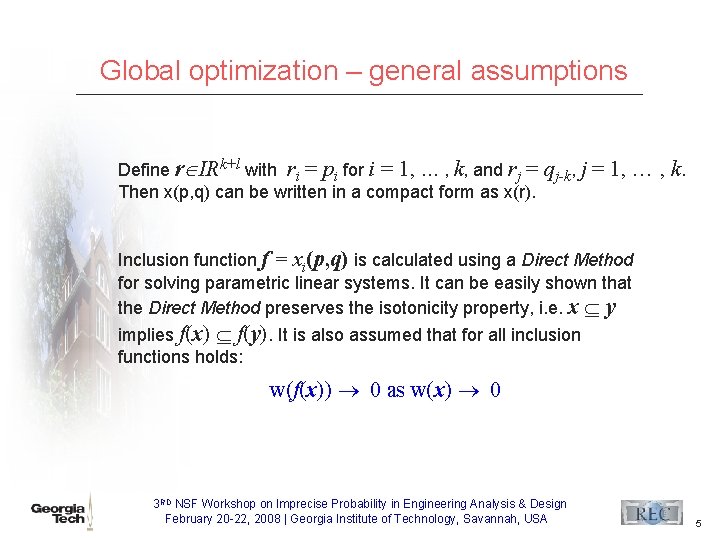
Global optimization – general assumptions Define r IRk+l with ri = pi for i = 1, , k, and rj = qj-k, j Then x(p, q) can be written in a compact form as x(r). = 1, , k. Inclusion function f = xi(p, q) is calculated using a Direct Method for solving parametric linear systems. It can be easily shown that the Direct Method preserves the isotonicity property, i. e. x y implies f(x) f(y). It is also assumed that for all inclusion functions holds: w(f(x)) 0 as w(x) 0 3 RD NSF Workshop on Imprecise Probability in Engineering Analysis & Design February 20 -22, 2008 | Georgia Institute of Technology, Savannah, USA 5

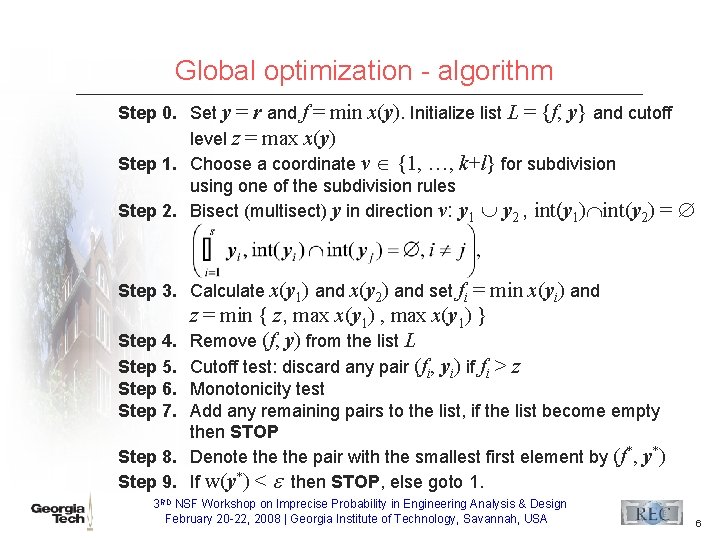
Global optimization - algorithm Step 0. Set y = r and f = min x(y). Initialize list L = {f, y} and cutoff level z = max x(y) Step 1. Choose a coordinate v {1, , k+l} for subdivision using one of the subdivision rules Step 2. Bisect (multisect) y in direction v: y 1 y 2 , int(y 1) int(y 2) = Step 3. Calculate x(y 1) and x(y 2) and set fi = min x(yi) and z = min { z, max x(y 1) } Step 4. Remove (f, y) from the list L Step 5. Cutoff test: discard any pair (fi, yi) if fi > z Step 6. Monotonicity test Step 7. Add any remaining pairs to the list, if the list become empty then STOP Step 8. Denote the pair with the smallest first element by (f*, y*) Step 9. If w(y*) < then STOP, else goto 1. 3 RD NSF Workshop on Imprecise Probability in Engineering Analysis & Design February 20 -22, 2008 | Georgia Institute of Technology, Savannah, USA 6

Monotonicity test The monotonicity test is used to figure out whether the function f is strictly monotone in a whole subbox y x. Then, y cannot contain a global minimizer in its interior. Therefore, if f satisfies Monotonicity test is pefromed using the Method for Checking the Monotonicity (MCM). The MCM method is based on a Direct Method for solving parametric linear systems. Let f = x(p, q). Approximations of partial derivates are obtained by solving the following k+l parametric linear systems where x* is an approximation of the solution set S calculated using Direct method, and 3 RD NSF Workshop on Imprecise Probability in Engineering Analysis & Design February 20 -22, 2008 | Georgia Institute of Technology, Savannah, USA 7

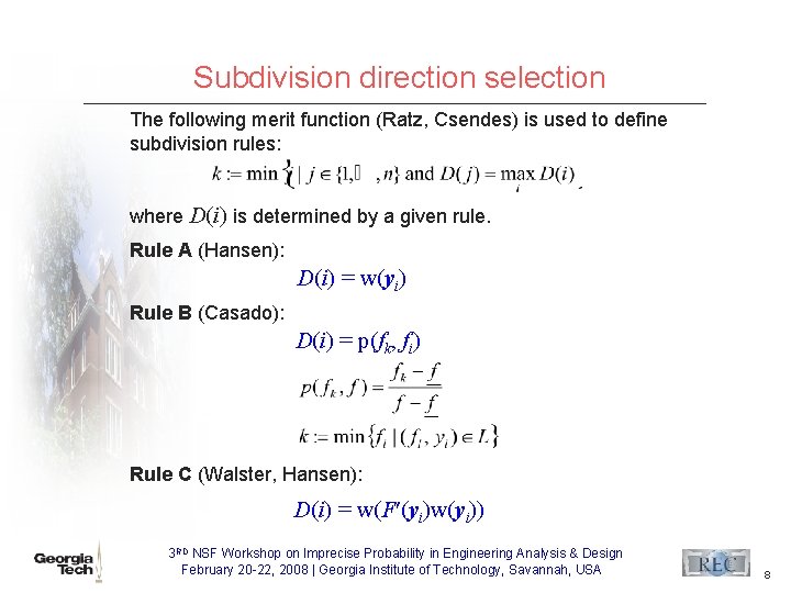
Subdivision direction selection The following merit function (Ratz, Csendes) is used to define subdivision rules: where D(i) is determined by a given rule. Rule A (Hansen): D(i) = w(yi) Rule B (Casado): D(i) = p(fk, fi) Rule C (Walster, Hansen): D(i) = w(F (yi)w(yi)) 3 RD NSF Workshop on Imprecise Probability in Engineering Analysis & Design February 20 -22, 2008 | Georgia Institute of Technology, Savannah, USA 8

Example 1 Young’s modulus Y = 7. 0 1010[Pa] Cross section aresa C = 0. 003[m 2] Length L = 2[m] Loads P 1 = P 2 = P 3 = 30[k. N] The stiffness of all bars is uncertain by 5% 3 RD NSF Workshop on Imprecise Probability in Engineering Analysis & Design February 20 -22, 2008 | Georgia Institute of Technology, Savannah, USA 9

Results – nodes displacements n x lb[ 10 -5] x ub[ 10 -5] n x lb[ 10 -5] x lb[ 10 -5 u 1 -32. 53 -29. 27 12 3. 90 4. 67 2 -1. 61 -1, 45 13 -16. 23 -14. 67 3 -26. 45 -23. 93 14 3. 18 3. 87 4 -2. 41 -2. 17 15 -3. 63 -2. 96 5 -15. 78 -14. 27 16 3. 18 3. 87 6 -1. 69 -1. 37 17 -0. 05 7 -4. 08 -3. 37 18 2. 35 3. 02 8 -0. 96 -0. 57 19 -0. 46 -0. 40 9 0. 36 0. 50 20 0. 85 1. 47 10 3. 90 4. 67 21 -2. 78 -2. 09 11 -26. 45 -23. 93 result of the Global Optimization = result of the Evolutionary Algorithm 3 RD NSF Workshop on Imprecise Probability in Engineering Analysis & Design February 20 -22, 2008 | Georgia Institute of Technology, Savannah, USA 10

Example 2 Young’s modulus Y = 2. 1 1011[Pa] Cross section aresa C = 0. 004[m 2] Length L = 2[m] Loads P 1 = 80[k. N], P 2 = 120[k. N] The stiffness of thick bars is uncertain by 5% result of the Global Optimization = result of the Evolutionary Algorithm 3 RD NSF Workshop on Imprecise Probability in Engineering Analysis & Design February 20 -22, 2008 | Georgia Institute of Technology, Savannah, USA 11

Conclusions ¥ Global Optimization Method can be succesfully used to approximate hull solution of parametric linear systems ¥ Monotonicity test significantly improves the convergence of Global Optimization ¥ Multidivision and different rules for subdivision directions have no influence on the convergence of the Global Optimization, they are computationally very expensive ¥ In future work we will try combine different methods for solving parametric linear systems 3 RD NSF Workshop on Imprecise Probability in Engineering Analysis & Design February 20 -22, 2008 | Georgia Institute of Technology, Savannah, USA 12