On the Performance of Parametric Polymorphism in Maple

On the Performance of Parametric Polymorphism in Maple Laurentiu Dragan Stephen M. Watt Ontario Research Centre for Computer Algebra University of Western Ontario Maple Conference 2006

Outline n n n Parametric Polymorphism Sci. Mark Sci. GMark A Maple Version of Sci. GMark Results Conclusions

Parametric Polymorphism n n Type Polymorphism – Allows a single definition of a function to be used with different types of data Parametric Polymorphism – A form of polymophism where the code does not use any specific type information – Instances with type parameters n n n Increasing popularity – C++, C#, Java Code reusability and reliability Generic Libraries – STL, Boost, NTL, Lin. Box, Sum-IT (Aldor)

Sci. Mark n National Institute of Standards and Technology – http: //math. nist. gov/scimark 2 n Consists of five kernels: 1. Fast Fourier transform – – – One-dimensional transform of 1024 complex numbers Each complex number 2 consecutive entries in the array Exercises complex arithmetic, non-constant memory references and trigonometric functions

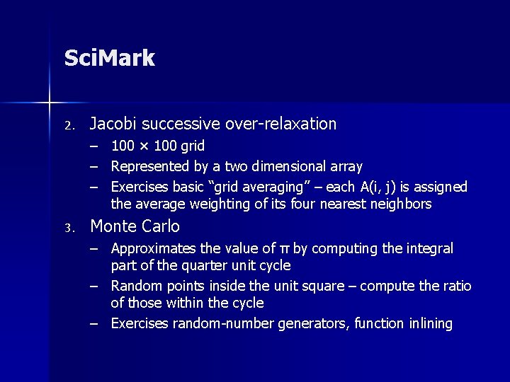
Sci. Mark 2. Jacobi successive over-relaxation – 100 × 100 grid – Represented by a two dimensional array – Exercises basic “grid averaging” – each A(i, j) is assigned the average weighting of its four nearest neighbors 3. Monte Carlo – Approximates the value of π by computing the integral part of the quarter unit cycle – Random points inside the unit square – compute the ratio of those within the cycle – Exercises random-number generators, function inlining

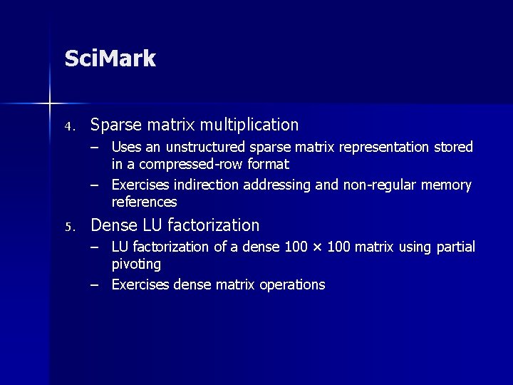
Sci. Mark 4. Sparse matrix multiplication – Uses an unstructured sparse matrix representation stored in a compressed-row format – Exercises indirection addressing and non-regular memory references 5. Dense LU factorization – LU factorization of a dense 100 × 100 matrix using partial pivoting – Exercises dense matrix operations

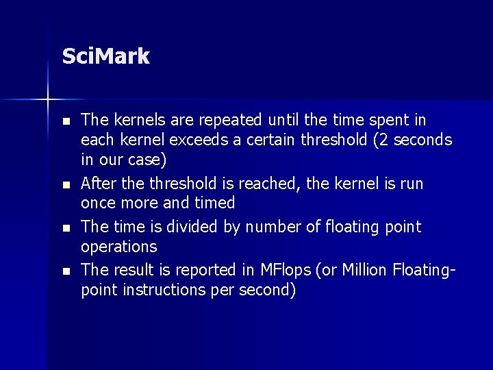
Sci. Mark n n The kernels are repeated until the time spent in each kernel exceeds a certain threshold (2 seconds in our case) After the threshold is reached, the kernel is run once more and timed The time is divided by number of floating point operations The result is reported in MFlops (or Million Floatingpoint instructions per second)

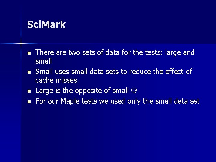
Sci. Mark n n There are two sets of data for the tests: large and small Small uses small data sets to reduce the effect of cache misses Large is the opposite of small For our Maple tests we used only the small data set

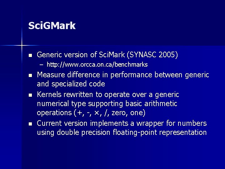
Sci. GMark n Generic version of Sci. Mark (SYNASC 2005) – http: //www. orcca. on. ca/benchmarks n n n Measure difference in performance between generic and specialized code Kernels rewritten to operate over a generic numerical type supporting basic arithmetic operations (+, -, ×, /, zero, one) Current version implements a wrapper for numbers using double precision floating-point representation

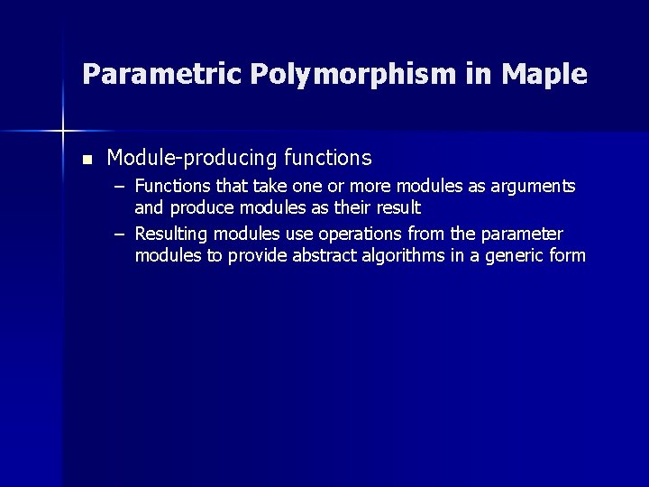
Parametric Polymorphism in Maple n Module-producing functions – Functions that take one or more modules as arguments and produce modules as their result – Resulting modules use operations from the parameter modules to provide abstract algorithms in a generic form

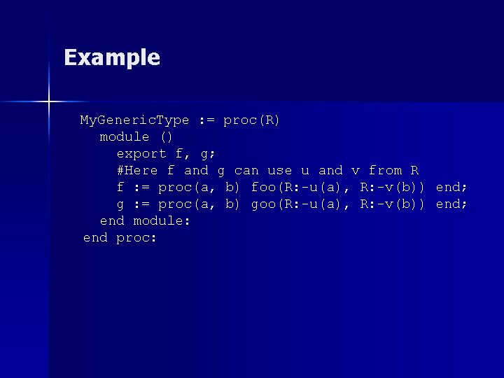
Example My. Generic. Type : = proc(R) module () export f, g; #Here f and g can use u and v from R f : = proc(a, b) foo(R: -u(a), R: -v(b)) end; g : = proc(a, b) goo(R: -u(a), R: -v(b)) end; end module: end proc:

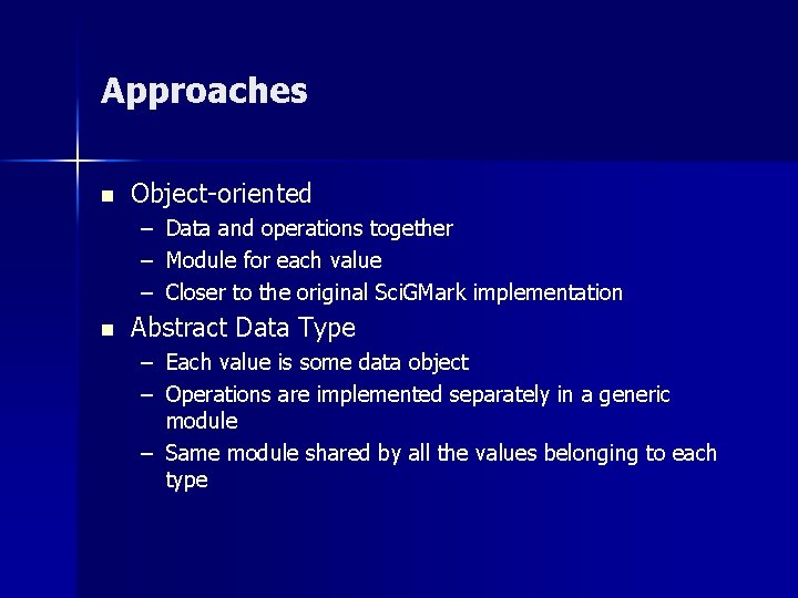
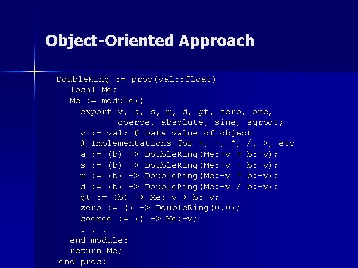
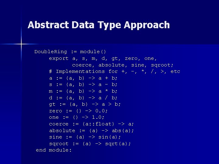
Approaches n Object-oriented – Data and operations together – Module for each value – Closer to the original Sci. GMark implementation n Abstract Data Type – Each value is some data object – Operations are implemented separately in a generic module – Same module shared by all the values belonging to each type

Object-Oriented Approach Double. Ring : = proc(val: : float) local Me; Me : = module() export v, a, s, m, d, gt, zero, one, coerce, absolute, sine, sqroot; v : = val; # Data value of object # Implementations for +, -, *, /, >, etc a : = (b) -> Double. Ring(Me: -v + b: -v); s : = (b) -> Double. Ring(Me: -v – b: -v); m : = (b) -> Double. Ring(Me: -v * b: -v); d : = (b) -> Double. Ring(Me: -v / b: -v); gt : = (b) -> Me: -v > b: -v; zero : = () -> Double. Ring(0. 0); coerce : = () -> Me: -v; . . . end module: return Me; end proc:

Object-Oriented Approach n n n Previous example simulates object-oriented approach by storing the value in the module The exports a, s, m, d correspond to basic arithmetic operations We chose names other than the standard +, -, ×, / for two reasons: – The code looks similar to the original Sci. GMark (Java does not have operator overloading) – It is not very easy to overload operators in Maple n Functions like sine and sqroot are used by the FFT algorithm to replace complex operations

Abstract Data Type Approach Double. Ring : = module() export a, s, m, d, gt, zero, one, coerce, absolute, sine, sqroot; # Implementations for +, -, *, /, >, etc a : = (a, b) -> a + b; s : = (a, b) -> a – b; m : = (a, b) -> a * b; d : = (a, b) -> a / b; gt : = (a, b) -> a > b; zero : = () -> 0. 0; one : = () -> 1. 0; coerce : = (a: : float) -> a; absolute : = (a) -> abs(a); sine : = (a) -> sin(a); sqroot : = (a) -> sqrt(a); end module:

Abstract Data Type Approach n n Module does not store data, provides only the operations As a convention one must coerce the float type to the representation used by this module In this case the representation is exactly float Double. Ring module created only once for each kernel

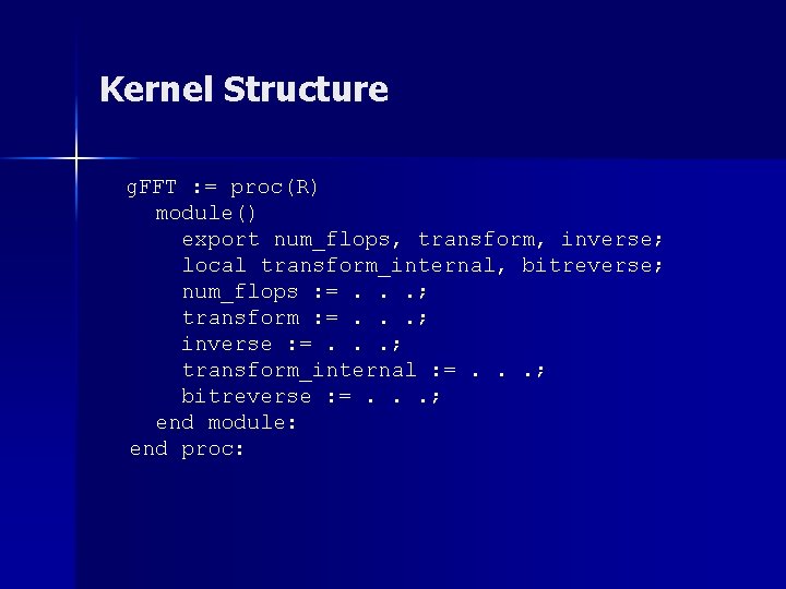
Kernels n n Each Sci. GMark kernel exports an implementation of its algorithm and a function to compute the estimated floating point operations Each kernel is parametrized by a module R, that abstracts the numerical type

Kernel Structure g. FFT : = proc(R) module() export num_flops, transform, inverse; local transform_internal, bitreverse; num_flops : =. . . ; transform : =. . . ; inverse : =. . . ; transform_internal : =. . . ; bitreverse : =. . . ; end module: end proc:

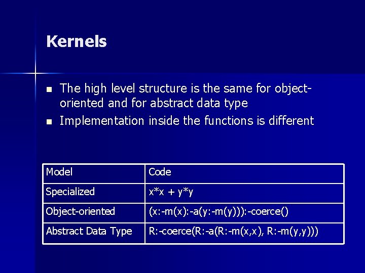
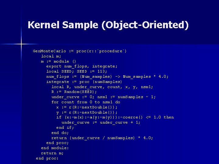
Kernels n n The high level structure is the same for objectoriented and for abstract data type Implementation inside the functions is different Model Code Specialized x*x + y*y Object-oriented (x: -m(x): -a(y: -m(y))): -coerce() Abstract Data Type R: -coerce(R: -a(R: -m(x, x), R: -m(y, y)))

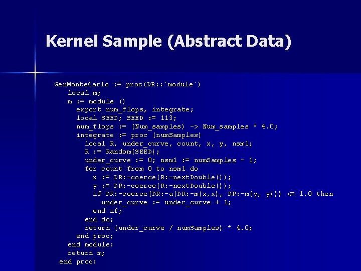
Kernel Sample (Abstract Data) Gen. Monte. Carlo : = proc(DR: : `module`) local m; m : = module () export num_flops, integrate; local SEED; SEED : = 113; num_flops : = (Num_samples) -> Num_samples * 4. 0; integrate : = proc (num. Samples) local R, under_curve, count, x, y, nsm 1; R : = Random(SEED); under_curve : = 0; nsm 1 : = num. Samples - 1; for count from 0 to nsm 1 do x : = DR: -coerce(R: -next. Double()); y : = DR: -coerce(R: -next. Double()); if DR: -coerce(DR: -a(DR: -m(x, x), DR: -m(y, y))) <= 1. 0 then under_curve : = under_curve + 1; end if; end do; return (under_curve / num. Samples) * 4. 0; end proc; end module: return m; end proc:

Kernel Sample (Object-Oriented) Gen. Monte. Carlo : = proc(r: : `procedure`) local m; m : = module () export num_flops, integrate; local SEED; SEED : = 113; num_flops : = (Num_samples) -> Num_samples * 4. 0; integrate : = proc (num. Samples) local R, under_curve, count, x, y, nsm 1; R : = Random(SEED); under_curve : = 0; nsm 1 : = num. Samples - 1; for count from 0 to nsm 1 do x : = r(R: -next. Double()); y : = r(R: -next. Double()); if (x: -m(x): -a(y: -m(y))): -coerce() <= 1. 0 then under_curve : = under_curve + 1; end if; end do; return (under_curve / num. Samples) * 4. 0; end proc; end module: return m; end proc:

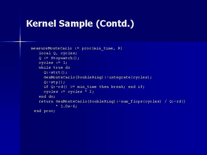
Kernel Sample (Contd. ) measure. Monte. Carlo : = proc(min_time, R) local Q, cycles; Q : = Stopwatch(); cycles : = 1; while true do Q: -strt(); Gen. Monte. Carlo(Double. Ring): -integrate(cycles); Q: -stp(); if Q: -rd() >= min_time then break; end if; cycles : = cycles * 2; end do; return Gen. Monte. Carlo(Double. Ring): -num_flops(cycles) / Q: -rd() * 1. 0 e-6; end proc;

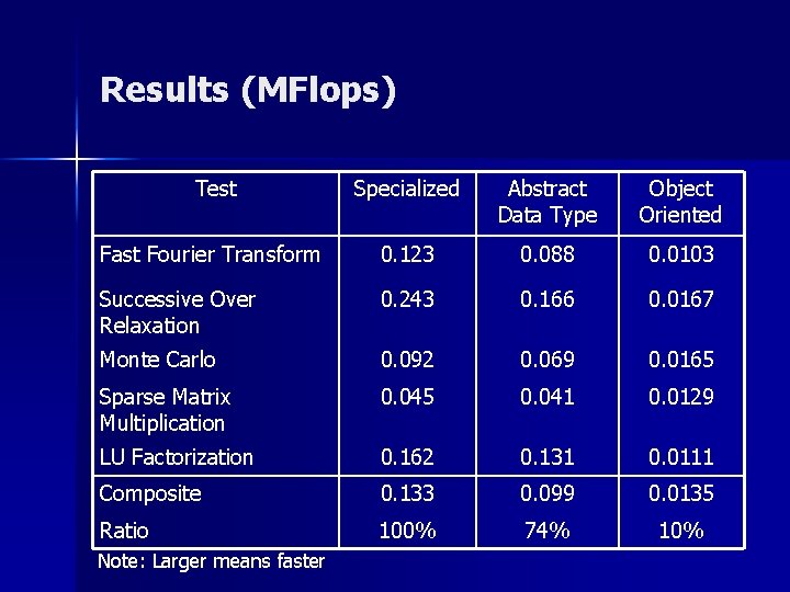
Results (MFlops) Test Specialized Abstract Data Type Object Oriented Fast Fourier Transform 0. 123 0. 088 0. 0103 Successive Over Relaxation 0. 243 0. 166 0. 0167 Monte Carlo 0. 092 0. 069 0. 0165 Sparse Matrix Multiplication 0. 045 0. 041 0. 0129 LU Factorization 0. 162 0. 131 0. 0111 Composite 0. 133 0. 099 0. 0135 Ratio 100% 74% 10% Note: Larger means faster

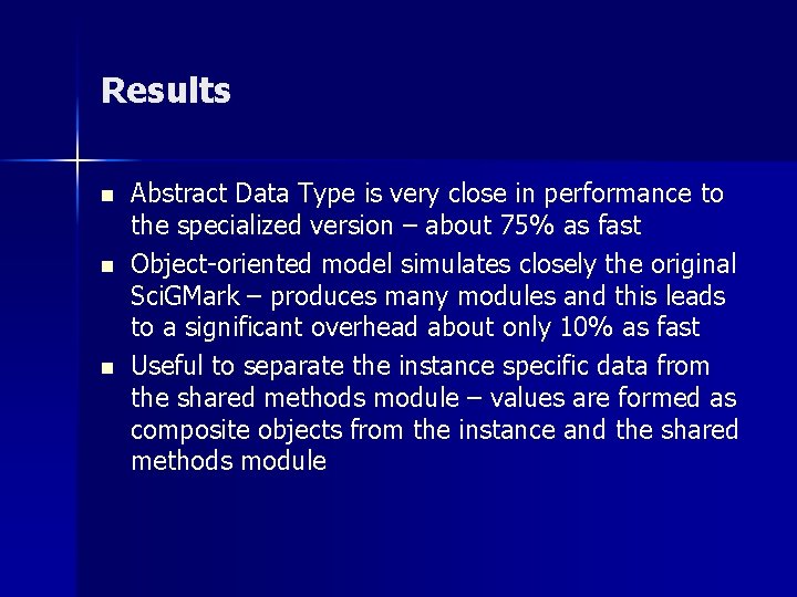
Results n n n Abstract Data Type is very close in performance to the specialized version – about 75% as fast Object-oriented model simulates closely the original Sci. GMark – produces many modules and this leads to a significant overhead about only 10% as fast Useful to separate the instance specific data from the shared methods module – values are formed as composite objects from the instance and the shared methods module

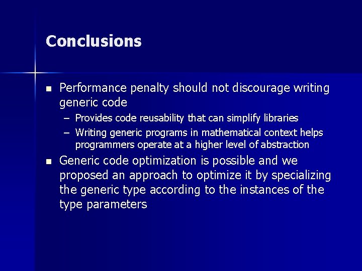
Conclusions n Performance penalty should not discourage writing generic code – Provides code reusability that can simplify libraries – Writing generic programs in mathematical context helps programmers operate at a higher level of abstraction n Generic code optimization is possible and we proposed an approach to optimize it by specializing the generic type according to the instances of the type parameters

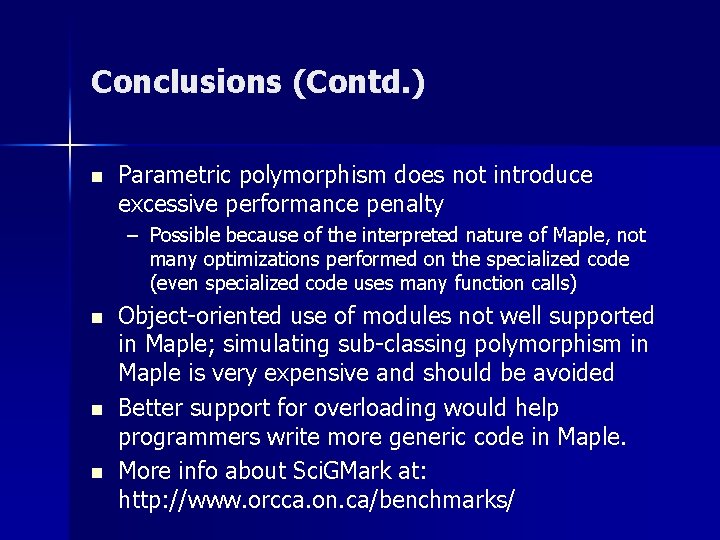
Conclusions (Contd. ) n Parametric polymorphism does not introduce excessive performance penalty – Possible because of the interpreted nature of Maple, not many optimizations performed on the specialized code (even specialized code uses many function calls) n n n Object-oriented use of modules not well supported in Maple; simulating sub-classing polymorphism in Maple is very expensive and should be avoided Better support for overloading would help programmers write more generic code in Maple. More info about Sci. GMark at: http: //www. orcca. on. ca/benchmarks/

Acknowledgments n n ORCCA members Maple. Soft