On the Flow Through Bering Strait A Synthesis

On the Flow Through Bering Strait: A Synthesis of Model Results and Observations Jaclyn Clement Kinney 1, Wieslaw Maslowski 1, Mike Steele 2, Yevgeny Aksenov 3, Beverly de Cuevas 3, Jaromir Jakacki 4, An Nguyen 5, Robert Osinski 1, Rebecca Woodgate 2, Jinlun Zhang 2 1 Naval Postgraduate School, Monterey, CA 2 Applied Physics Laboratory, Univ. Washington, Seattle, WA 3 National Oceanography Centre, Southampton, UK 4 Institute of Oceanology, Polish Academy of Sciences, Sopot, Poland 5 Jet Propulsion Laboratory, Pasadena, CA Sponsored by NSF/AOMIP IPY Oslo Science Conference, Norway

Importance of Bering Strait: - only Pacific connection to the Chukchi Sea and greater Arctic Ocean - political boundary restricts access - challenge to observationalists and modelers - important for maintenance of Arctic Ocean halocline, ice edge position, transports through Fram Strait, and freshwater budgets in the Nordic Seas Primary goal of this work: Intercomparison of the volume, heat and freshwater fluxes through Bering Strait. Courtesy NASA/JPL
 •")
Observations in Bering Strait Observational results provided by UW (Woodgate et al. ) • moored instruments placed ~10 m above the bottom (A 1, A 2, A 3) • velocity, T, S: eastern channel and north of the strait (since 1991) • very limited access to the western channel of Bering Strait – Russian waters (intermittent data during 1990 -1994) • fluxes extrapolated from point measurements (e. g. Woodgate et al. , 2005) • additional moorings added thanks to recent collaboration between the US and Russia (light blue dots; data no yet publicly available)
 BESTMAS (http:")
Participating modeling groups UW models: PIOMAS (http: //psc. apl. washington. edu/IDAO/model. html) BESTMAS (http: //psc. apl. washington. edu/BEST. html) • POP (ocean) and TED (ice) • NCEP/NCAR reanalysis forcing • horizontal resolution is ~22 km (PIOMAS) and ~7 km (BESTMAS), 30 vertical levels • new BESTMAS run with min. ocean depth of 15 m (instead of 30 m) and widened Bering Strait ECCO 2 (http: //ecco 2. org/) • MITgcm (ocean) and (ice) • Japanese 25 -year Re. Analysis (JRA-25) forcing • 18 km horizontal resolution, 50 vertical levels • 10 m minimum ocean depth ORCA (http: //www. noc. soton. ac. uk/nemo/) • ORCA 025 L 64 -N 102 - NEMO framework (ocean) and LIM 2 sea ice model: VP and 2 -layer Semtner thermodynamics • 6 -hourly ECMWF/CORE 2 -based DRAKAR Forcing Set (DFS 3) forcing • Horizontal grid: Global Arakawa C tri-polar, min 6 km (zonal) X 3. 1 km (meridional), max 27. 8 km, 64 vertical levels • 25 m minimum ocean depth NPS (NAME) (http: //www. oc. nps. edu/NAME/name. html) • based on POP (ocean) and Zhang-Hibler (ice); transitioning to CICE (ice) • daily ECMWF forcing • ~9 km horizontal resolution, 45 vertical levels, 10 m minimum ocean depth
 velocity across Bering Strait from 5 models • significant horizontal")
Long-term mean (1979 -2004) velocity across Bering Strait from 5 models • significant horizontal shear in all models • some vertical shear • highest velocity in eastern channel
 Velocity from ~10 m")
Monthly mean Velocity from models and observations A 2 (East) Velocity from ~10 m above the seafloor A 2 location in the deep part of the Eastern Channel Correlation coefficients between modeled and observed velocities range between 0. 69 – 0. 77

Comparison of model and data long-term means of velocity and volume transport model/d ata mean volume velocity transport BESTMAS 34. 0 0. 72 NPS 34. 1 0. 65 data 24. 8 0. 8+ ORCA 43. 2 1. 33 ECCO 2 39. 9 1. 07 PIOMAS 29. 5 0. 79 Higher resolution models (BESTMAS and NPS) have lower mean velocities and volume transport Lower resolution models tend to have higher mean velocities and volume transport

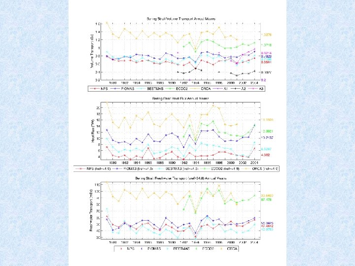
Volume, heat, and freshwater transports for model sections across Bering Strait data mean (1991 -2004) = 0. 80 Sv data mean (1991 -2004) = 6 TW data mean (1991 -2004) = 54 m. Sv

Annual Cycles of volume, heat and freshwater transport • strong annual cycles, as is typical of arctic seas • data shows the strongest annual cycle of volume • most models have a similarly-shaped annual cycle • heat flux peaks in August and is near zero in winter • freshwater peaks in midsummer

Comparison of the March mean velocity between the 9 -km and 2. 3 -km NPS model runs 1/12 o (9 km) NPS model 1/48 o (2. 3 km) NPS model • going to 2 km does not qualitatively change the structure of the flow and property transport across Bering Strait, however the flow is more realistic in high resolution • the range of velocity at the mooring location ~10 above the bottom can be large
 remain with accurate estimation")
Conclusions and future work • At present, uncertainties (? %) remain with accurate estimation of volume transport through Bering Strait • Other property transports will be affected by uncertainty in volume transport § High resolution models produce lower values of the transport, while lower resolution models produce higher values § Moving to higher horizontal resolution (2 km) does not qualitatively change the structure of the flow and property transport across Bering Strait, however smaller scale features are better represented § An expanded array of observations of vertical and horizontal structure and their temporal evolution in Bering Strait is needed to better constrain models and narrow uncertainty § this is currently underway, with more moorings in the strait § availability of processed data for model intercomparison

 combined with AVHRR SSTs Woodgate et al. , 2010 GRL recent")
Moored observations (near-bottom) combined with AVHRR SSTs Woodgate et al. , 2010 GRL recent temperature and associated heat flux increase in 2007 (due to including AVHRR SST in estimates) – how would other surface estimates change total fluxes?
 • highest speeds")
Velocity contours from current meter data (Coachman et al. , 1975) • highest speeds tend to be found in the eastern channel • the pattern of horizontal shear in the Bering Strait seems to be relatively invariant • a velocity minimum West of Fairway Rock • several cases of local flow reversal in the upper layer

Comparison of the 2 methods of volume transport calculation full model cross-section utilizing all points in horizontal and vertical velocity near-bottom at A 2 location multiplied by crosssectional area of 2. 6 km 2 (method used in Woodgate et al. , 2005 GRL) The observational method yields a volume transport that is 25% higher than the full model cross-section. (Clement et al. , 2005 DSRII) Using the observational method for other model results yields a volume transport that may be higher or lower than the full model crosssection…however it is never the same.
- Slides: 16