On the Constancy of Internet Path Properties Yin

On the Constancy of Internet Path Properties Yin Zhang Nick Duffield Vern Paxson Scott Shenker AT&T Labs – Research ACIRI {yzhang, duffield}@research. att. com {vern, shenker}@aciri. org ACM SIGCOMM Internet Measurement Workshop November, 2001 11/02/2001 IMW'2001 1

Talk Outline n n Motivation Three notions of constancy n n Constancy of three Internet path properties n n Mathematical Operational Predictive Packet loss Packet delays Throughput Conclusions 11/02/2001 IMW'2001 2

Motivation n Recent surge of interest in network measurement n n Mathematical modeling Operational procedures Adaptive applications Measurements are most valuable when the relevant network properties exhibit constancy n n Constancy: holds steady and does not change We will also use the term steady, when use of “constancy” would prove grammatically awkward 11/02/2001 IMW'2001 3

Mathematical Constancy n A dataset is mathematically steady if it can be described with a single time-invariant mathematical model. n n n Simplest form: IID – independent and identically distributed Key: finding the appropriate model Examples n Mathematical constancy n n Session arrivals are well described by a fix-rate Poisson process over time scales of 10 s of minutes to an hour [PF 95] Mathematical non-constancy n 11/02/2001 Session arrivals over larger time scales IMW'2001 4

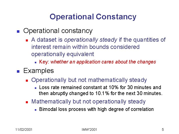
Operational Constancy n Operational constancy n A dataset is operationally steady if the quantities of interest remain within bounds considered operationally equivalent n n Key: whether an application cares about the changes Examples n Operationally but not mathematically steady n n Loss rate remained constant at 10% for 30 minutes and then abruptly changed to 10. 1% for the next 30 minutes. Mathematically but not operationally steady n 11/02/2001 Bimodal loss process with high degree of correlation IMW'2001 5

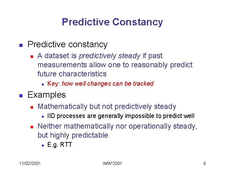
Predictive Constancy n Predictive constancy n A dataset is predictively steady if past measurements allow one to reasonably predict future characteristics n n Key: how well changes can be tracked Examples n Mathematically but not predictively steady n n IID processes are generally impossible to predict well Neither mathematically nor operationally steady, but highly predictable n 11/02/2001 E. g. RTT IMW'2001 6

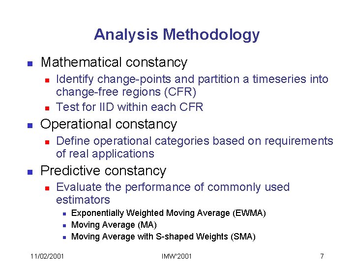
Analysis Methodology n Mathematical constancy n n n Operational constancy n n Identify change-points and partition a timeseries into change-free regions (CFR) Test for IID within each CFR Define operational categories based on requirements of real applications Predictive constancy n Evaluate the performance of commonly used estimators n n n 11/02/2001 Exponentially Weighted Moving Average (EWMA) Moving Average (MA) Moving Average with S-shaped Weights (SMA) IMW'2001 7

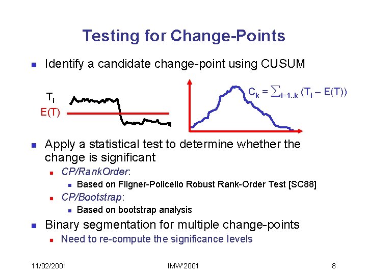
Testing for Change-Points n Identify a candidate change-point using CUSUM Ck = i=1. . k (Ti – E(T)) Ti E(T) n Apply a statistical test to determine whether the change is significant n CP/Rank. Order: n n CP/Bootstrap: n n Based on Fligner-Policello Robust Rank-Order Test [SC 88] Based on bootstrap analysis Binary segmentation for multiple change-points n Need to re-compute the significance levels 11/02/2001 IMW'2001 8

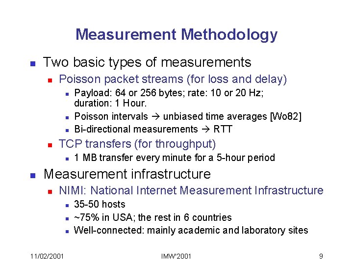
Measurement Methodology n Two basic types of measurements n Poisson packet streams (for loss and delay) n n TCP transfers (for throughput) n n Payload: 64 or 256 bytes; rate: 10 or 20 Hz; duration: 1 Hour. Poisson intervals unbiased time averages [Wo 82] Bi-directional measurements RTT 1 MB transfer every minute for a 5 -hour period Measurement infrastructure n NIMI: National Internet Measurement Infrastructure n n n 11/02/2001 35 -50 hosts ~75% in USA; the rest in 6 countries Well-connected: mainly academic and laboratory sites IMW'2001 9

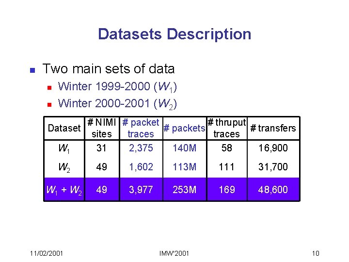
Datasets Description n Two main sets of data n n Winter 1999 -2000 (W 1) Winter 2000 -2001 (W 2) Dataset W 1 # NIMI # packet # thruput # packets # transfers sites traces 31 2, 375 140 M 58 16, 900 W 2 49 1, 602 113 M 111 31, 700 W 1 + W 2 49 3, 977 253 M 169 48, 600 11/02/2001 IMW'2001 10

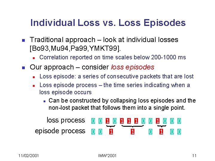
Individual Loss vs. Loss Episodes n Traditional approach – look at individual losses [Bo 93, Mu 94, Pa 99, YMKT 99]. n n Correlation reported on time scales below 200 -1000 ms Our approach – consider loss episodes n n Loss episode: a series of consecutive packets that are lost Loss episode process – the time series indicating when a loss episode occurs n Can be constructed by collapsing loss episodes and the non-lost packet that follows them into a single point. loss process 0 0 1 1 1 0 0 0 episode process 0 0 1 1 0 0 11/02/2001 IMW'2001 11

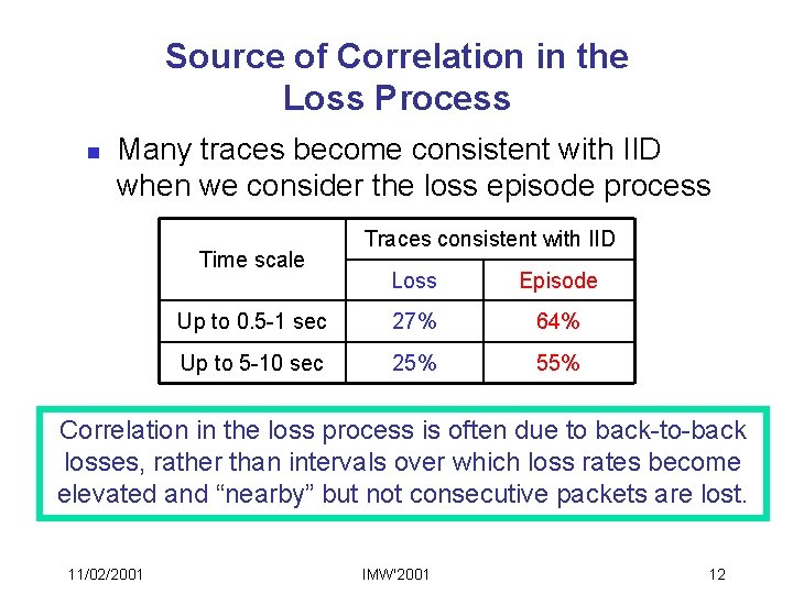
Source of Correlation in the Loss Process n Many traces become consistent with IID when we consider the loss episode process Time scale Traces consistent with IID Loss Episode Up to 0. 5 -1 sec 27% 64% Up to 5 -10 sec 25% 55% Correlation in the loss process is often due to back-to-back losses, rather than intervals over which loss rates become elevated and “nearby” but not consecutive packets are lost. 11/02/2001 IMW'2001 12

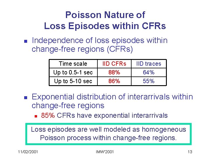
Poisson Nature of Loss Episodes within CFRs n n Independence of loss episodes within change-free regions (CFRs) Time scale Up to 0. 5 -1 sec IID CFRs 88% IID traces 64% Up to 5 -10 sec 86% 55% Exponential distribution of interarrivals within change-free regions n 85% CFRs have exponential interarrivals Loss episodes are well modeled as homogeneous Poisson process within change-free regions. 11/02/2001 IMW'2001 13

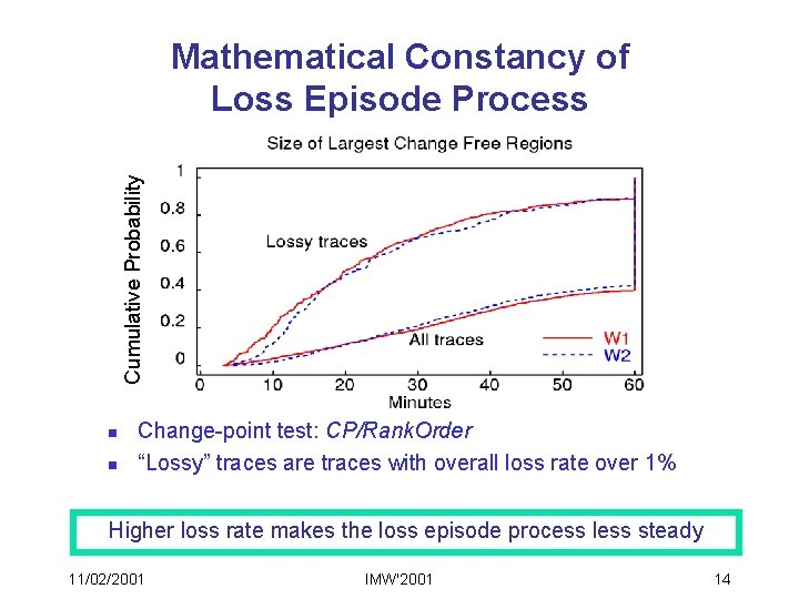
Cumulative Probability Mathematical Constancy of Loss Episode Process n n Change-point test: CP/Rank. Order “Lossy” traces are traces with overall loss rate over 1% Higher loss rate makes the loss episode process less steady 11/02/2001 IMW'2001 14

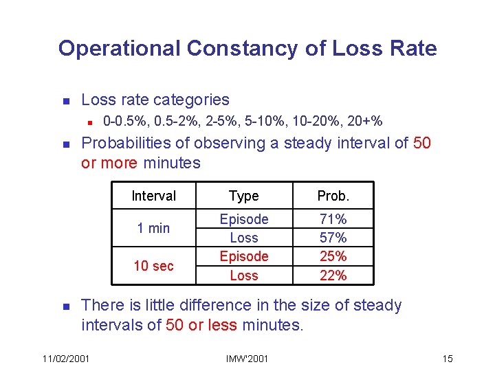
Operational Constancy of Loss Rate n Loss rate categories n n 0 -0. 5%, 0. 5 -2%, 2 -5%, 5 -10%, 10 -20%, 20+% Probabilities of observing a steady interval of 50 or more minutes Interval 1 min 10 sec n Type Prob. Episode Loss 71% 57% 25% 22% There is little difference in the size of steady intervals of 50 or less minutes. 11/02/2001 IMW'2001 15

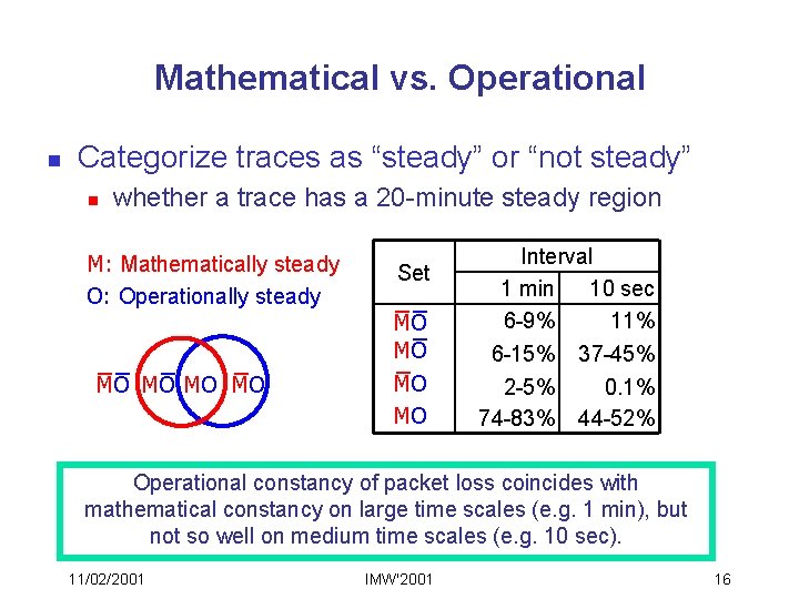
Mathematical vs. Operational n Categorize traces as “steady” or “not steady” n whether a trace has a 20 -minute steady region M: Mathematically steady O: Operationally steady MO ¯ ¯ MO MO ¯ Set MO ¯¯ MO Interval 1 min 10 sec 6 -9% 11% 6 -15% 37 -45% 2 -5% 0. 1% 74 -83% 44 -52% Operational constancy of packet loss coincides with mathematical constancy on large time scales (e. g. 1 min), but not so well on medium time scales (e. g. 10 sec). 11/02/2001 IMW'2001 16

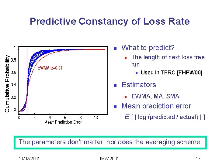
Predictive Constancy of Loss Rate Cumulative Probability n What to predict? n The length of next loss free run n n Estimators n n Used in TFRC [FHPW 00] EWMA, SMA Mean prediction error E [ | log (predicted / actual) | ] The parameters don’t matter, nor does the averaging scheme. 11/02/2001 IMW'2001 17

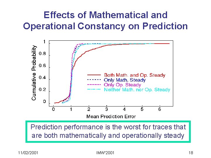
Cumulative Probability Effects of Mathematical and Operational Constancy on Prediction performance is the worst for traces that are both mathematically and operationally steady 11/02/2001 IMW'2001 18

Delay Constancy n Mathematical constancy n Delay “spikes” n A spike is identified when n R’ max{ K·R, 250 ms } (K = 2 or 4) where n n R’ is the new RTT measurement; R is the previous non-spike RTT measurement; The spike episode process is well described as Poisson within CFRs Body of RTT distribution (Median, IQR) n n 11/02/2001 Overall, less steady than loss Good agreement (90 -92%) with IID within CFRs IMW'2001 19

Delay Constancy (cont’d) n Operational constancy n Operational categories n 0 -0. 1 sec, 0. 1 -0. 2 sec, 0. 2 -0. 3 sec, 0. 3 -0. 8 sec, 0. 8+sec n n Not operationally steady n n n Based on ITU Recommendation G. 114 Over 50% traces have max steady regions under 10 min; 80% are under 20 minutes Predictive constancy n n All estimators perform similar Highly predictable in general 11/02/2001 IMW'2001 20

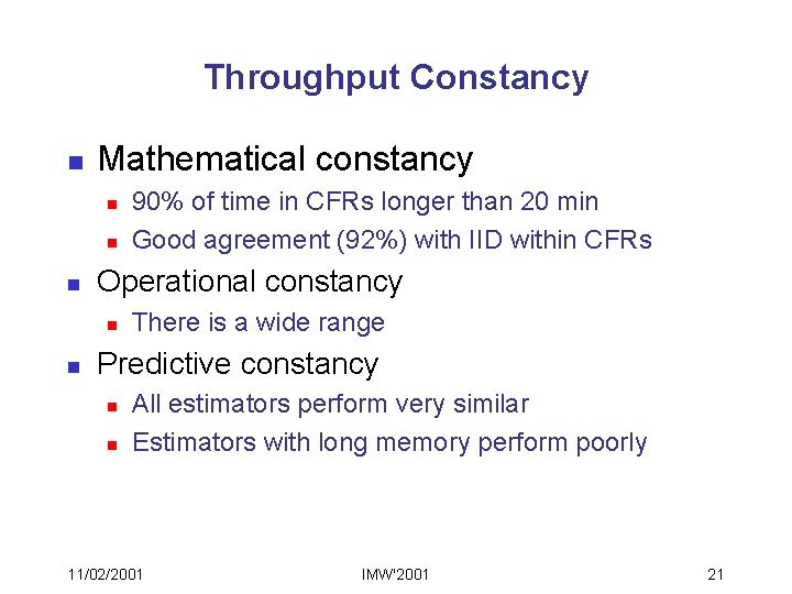
Throughput Constancy n Mathematical constancy n n n Operational constancy n n 90% of time in CFRs longer than 20 min Good agreement (92%) with IID within CFRs There is a wide range Predictive constancy n n All estimators perform very similar Estimators with long memory perform poorly 11/02/2001 IMW'2001 21

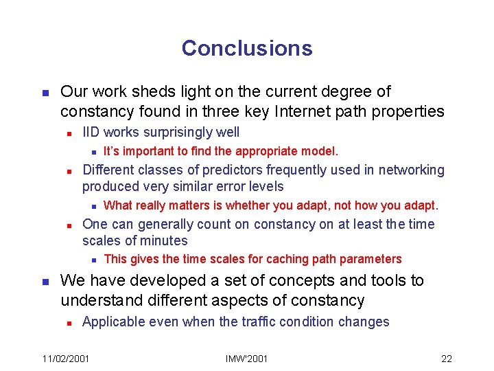
Conclusions n Our work sheds light on the current degree of constancy found in three key Internet path properties n IID works surprisingly well n n Different classes of predictors frequently used in networking produced very similar error levels n n What really matters is whether you adapt, not how you adapt. One can generally count on constancy on at least the time scales of minutes n n It’s important to find the appropriate model. This gives the time scales for caching path parameters We have developed a set of concepts and tools to understand different aspects of constancy n Applicable even when the traffic condition changes 11/02/2001 IMW'2001 22

Acknowledgments n n n Andrew Adams Matt Mathis Jamshid Mahdavi Lee Breslau Mark Allman NIMI volunteers 11/02/2001 IMW'2001 23