On the alternative approaches to ITRF formulation A





- Slides: 82

On the alternative approaches to ITRF formulation. A theoretical comparison. Athanasios Dermanis Department of Geodesy and Surveying Aristotle University of Thessaloniki

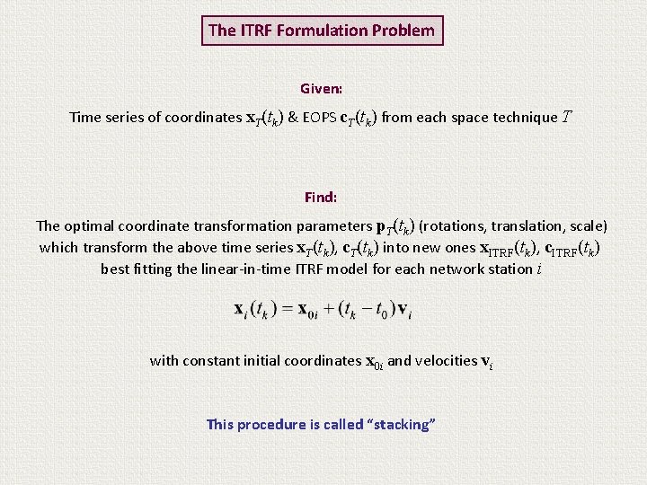
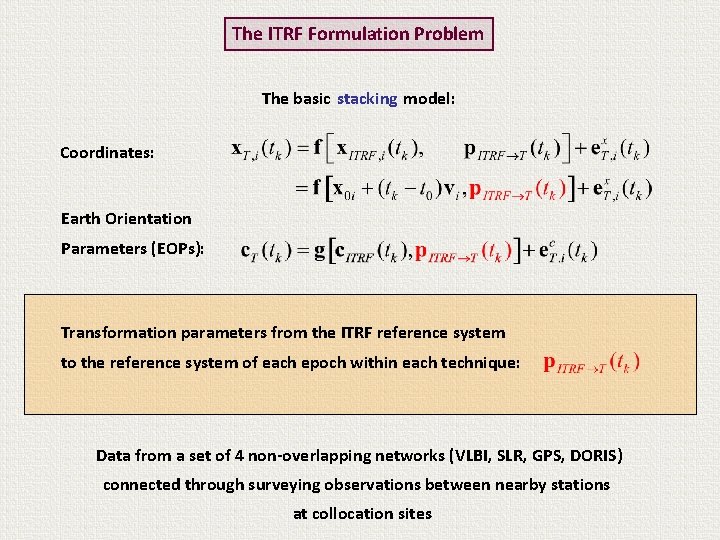
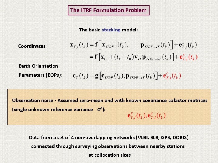
The ITRF Formulation Problem Given: Time series of coordinates x. T(tk) & EOPS c. T(tk) from each space technique T Find: The optimal coordinate transformation parameters p. T(tk) (rotations, translation, scale) which transform the above time series x. T(tk), c. T(tk) into new ones x. ITRF(tk), c. ITRF(tk) best fitting the linear-in-time ITRF model for each network station i with constant initial coordinates x 0 i and velocities vi This procedure is called “stacking”

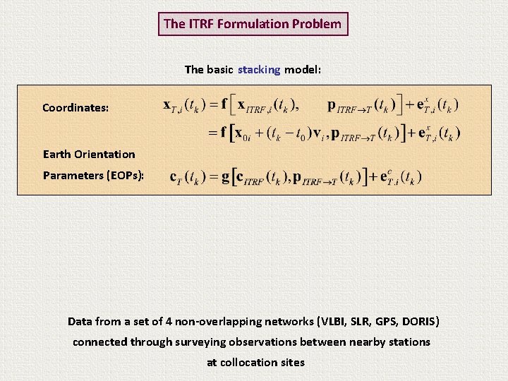
The ITRF Formulation Problem The basic stacking model: Coordinates: Earth Orientation Parameters (EOPs): Data from a set of 4 non-overlapping networks (VLBI, SLR, GPS, DORIS) connected through surveying observations between nearby stations at collocation sites

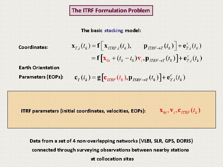
The ITRF Formulation Problem The basic stacking model: Coordinates: Earth Orientation Parameters (EOPs): ITRF parameters (initial coordinates, velocities, EOPs): Data from a set of 4 non-overlapping networks (VLBI, SLR, GPS, DORIS) connected through surveying observations between nearby stations at collocation sites

The ITRF Formulation Problem The basic stacking model: Coordinates: Earth Orientation Parameters (EOPs): Transformation parameters from the ITRF reference system to the reference system of each epoch within each technique: Data from a set of 4 non-overlapping networks (VLBI, SLR, GPS, DORIS) connected through surveying observations between nearby stations at collocation sites

The ITRF Formulation Problem The basic stacking model: Coordinates: Earth Orientation Parameters (EOPs): Observation noise - Assumed zero-mean and with known covariance cofactor matrices (single unknown reference variance 2): Data from a set of 4 non-overlapping networks (VLBI, SLR, GPS, DORIS) connected through surveying observations between nearby stations at collocation sites

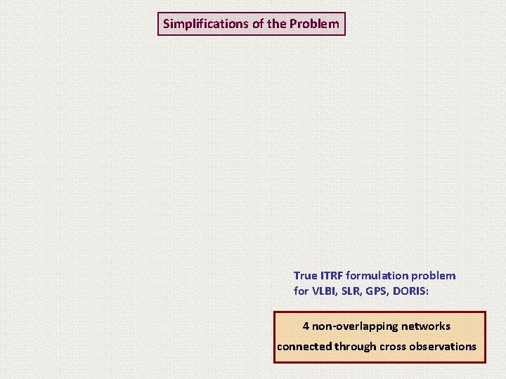
Simplifications of the Problem True ITRF formulation problem for VLBI, SLR, GPS, DORIS: 4 non-overlapping networks connected through cross observations

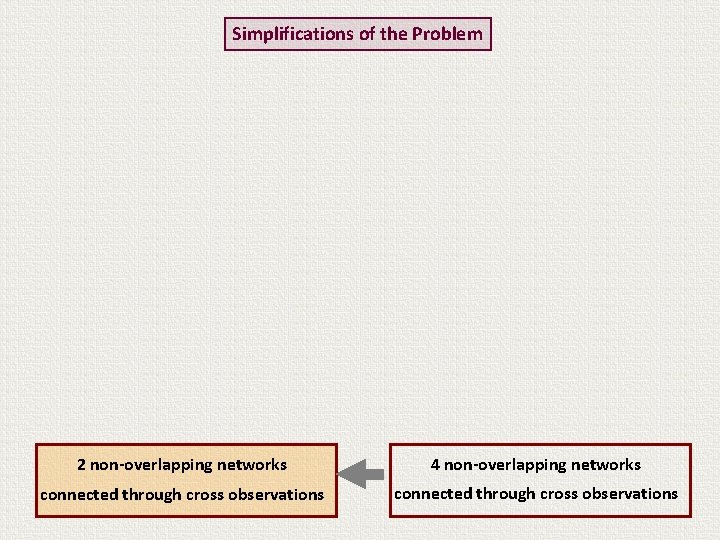
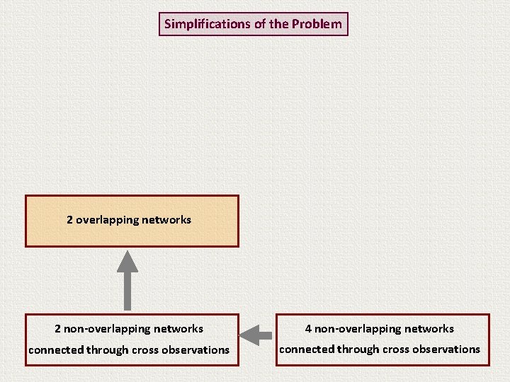
Simplifications of the Problem 2 non-overlapping networks 4 non-overlapping networks connected through cross observations

Simplifications of the Problem 2 overlapping networks 2 non-overlapping networks 4 non-overlapping networks connected through cross observations

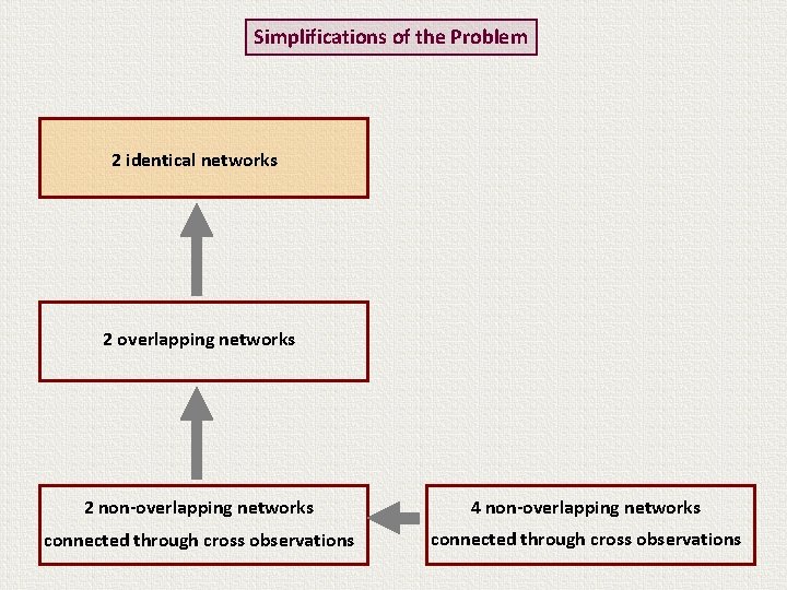
Simplifications of the Problem 2 identical networks 2 overlapping networks 2 non-overlapping networks 4 non-overlapping networks connected through cross observations

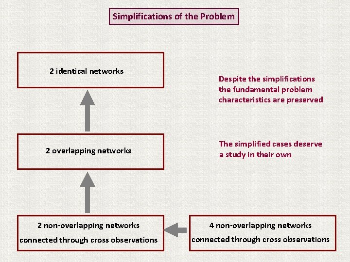
Simplifications of the Problem 2 identical networks 2 overlapping networks Despite the simplifications the fundamental problem characteristics are preserved The simplified cases deserve a study in their own 2 non-overlapping networks 4 non-overlapping networks connected through cross observations

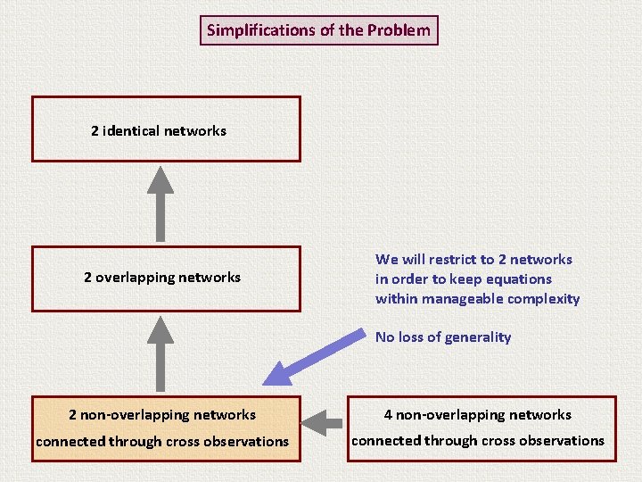
Simplifications of the Problem 2 identical networks 2 overlapping networks We will restrict to 2 networks in order to keep equations within manageable complexity No loss of generality 2 non-overlapping networks 4 non-overlapping networks connected through cross observations

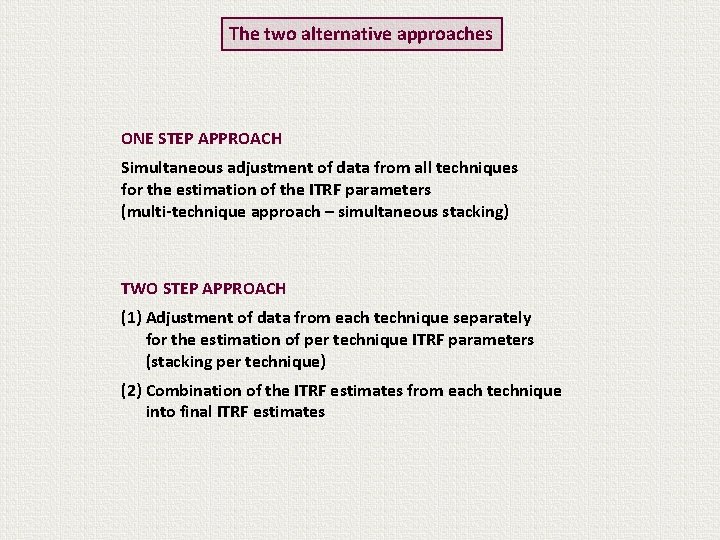
The two alternative approaches ONE STEP APPROACH Simultaneous adjustment of data from all techniques for the estimation of the ITRF parameters (multi-technique approach – simultaneous stacking) TWO STEP APPROACH (1) Adjustment of data from each technique separately for the estimation of per technique ITRF parameters (stacking per technique) (2) Combination of the ITRF estimates from each technique into final ITRF estimates

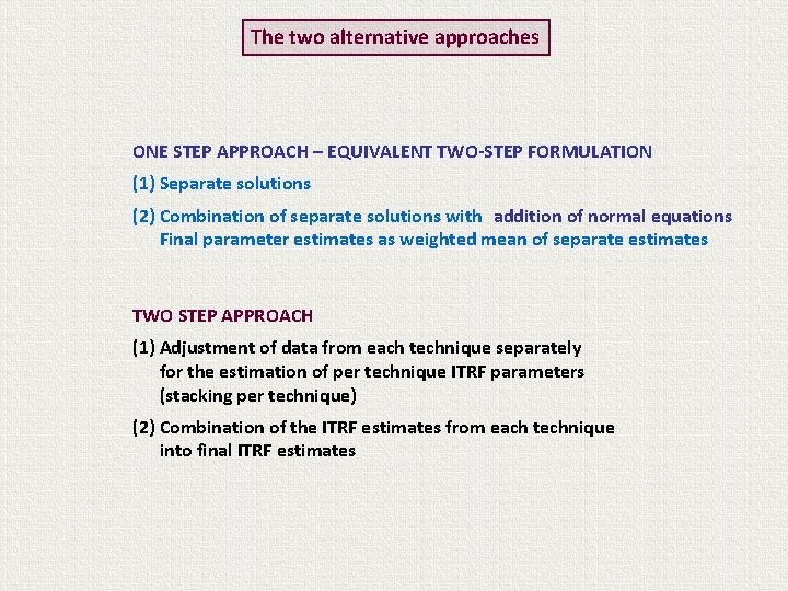
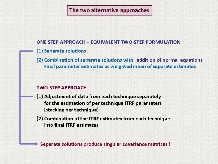
The two alternative approaches ONE STEP APPROACH – EQUIVALENT TWO-STEP FORMULATION (1) Separate solutions (2) Combination of separate solutions with addition of normal equations Final parameter estimates as weighted mean of separate estimates TWO STEP APPROACH (1) Adjustment of data from each technique separately for the estimation of per technique ITRF parameters (stacking per technique) (2) Combination of the ITRF estimates from each technique into final ITRF estimates

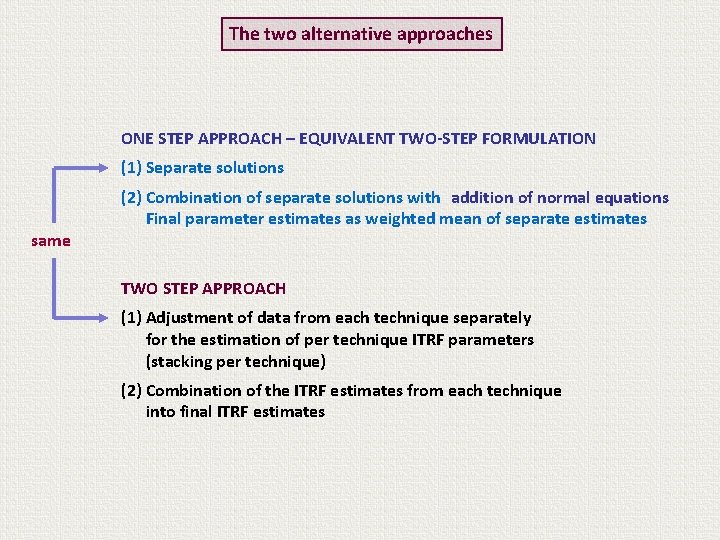
The two alternative approaches ONE STEP APPROACH – EQUIVALENT TWO-STEP FORMULATION (1) Separate solutions same (2) Combination of separate solutions with addition of normal equations Final parameter estimates as weighted mean of separate estimates TWO STEP APPROACH (1) Adjustment of data from each technique separately for the estimation of per technique ITRF parameters (stacking per technique) (2) Combination of the ITRF estimates from each technique into final ITRF estimates

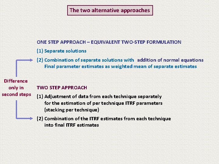
The two alternative approaches ONE STEP APPROACH – EQUIVALENT TWO-STEP FORMULATION (1) Separate solutions (2) Combination of separate solutions with addition of normal equations Final parameter estimates as weighted mean of separate estimates Difference only in second steps TWO STEP APPROACH (1) Adjustment of data from each technique separately for the estimation of per technique ITRF parameters (stacking per technique) (2) Combination of the ITRF estimates from each technique into final ITRF estimates

The two alternative approaches ONE STEP APPROACH – EQUIVALENT TWO-STEP FORMULATION (1) Separate solutions (2) Combination of separate solutions with addition of normal equations Final parameter estimates as weighted mean of separate estimates TWO STEP APPROACH (1) Adjustment of data from each technique separately for the estimation of per technique ITRF parameters (stacking per technique) (2) Combination of the ITRF estimates from each technique into final ITRF estimates Separate solutions produce singular covariance matrices !

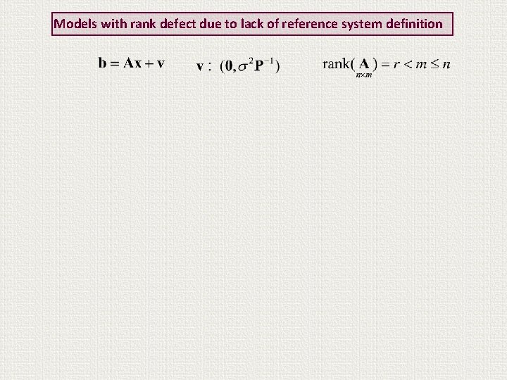
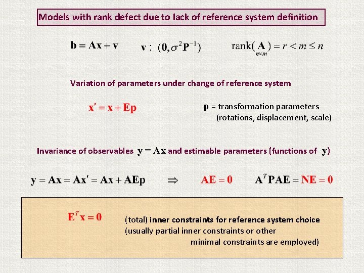
Models with rank defect due to lack of reference system definition

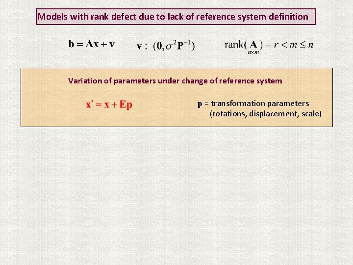
Models with rank defect due to lack of reference system definition Variation of parameters under change of reference system p = transformation parameters (rotations, displacement, scale)

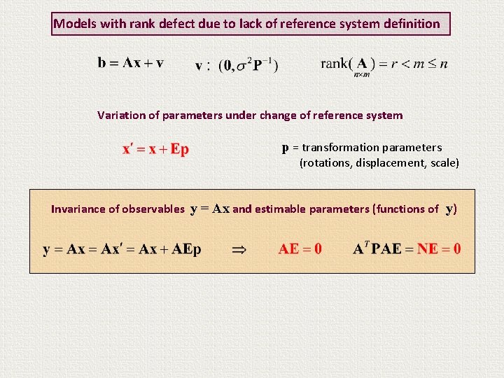
Models with rank defect due to lack of reference system definition Variation of parameters under change of reference system p = transformation parameters (rotations, displacement, scale) Invariance of observables y = Ax and estimable parameters (functions of y)

Models with rank defect due to lack of reference system definition Variation of parameters under change of reference system p = transformation parameters (rotations, displacement, scale) Invariance of observables y = Ax and estimable parameters (functions of y) (total) inner constraints for reference system choice (usually partial inner constraints or other minimal constraints are employed)

Two identical networks This case does not apply to the ITRF formulation problem but has an interest of its own for other network applications

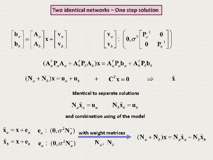
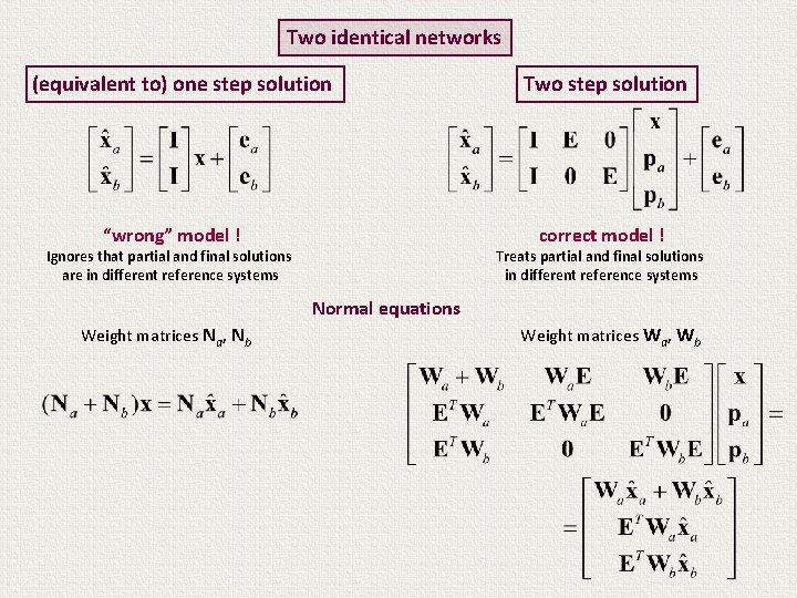
Two identical networks – One step solution Identical to separate solutions and combination using of the model with weight matrices

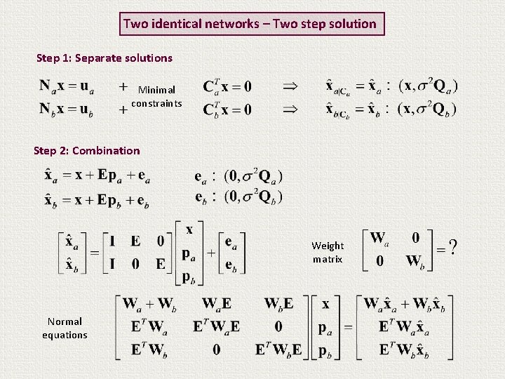
Two identical networks – Two step solution Step 1: Separate solutions Minimal constraints Step 2: Combination Weight matrix Normal equations

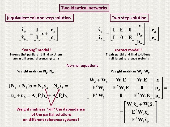
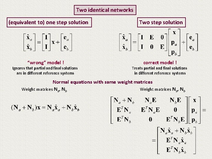
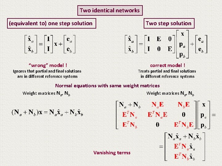
Two identical networks (equivalent to) one step solution “wrong” model ! Two step solution correct model ! Ignores that partial and final solutions are in different reference systems Treats partial and final solutions in different reference systems Normal equations Weight matrices Na, Nb Weight matrices Wa, Wb

Two identical networks (equivalent to) one step solution “wrong” model ! Two step solution correct model ! Ignores that partial and final solutions are in different reference systems Treats partial and final solutions in different reference systems Normal equations Weight matrices Na, Nb Weight matrices “kill” the dependence of the partial solutions on different reference systems ! Weight matrices Wa, Wb

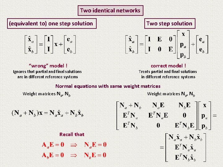
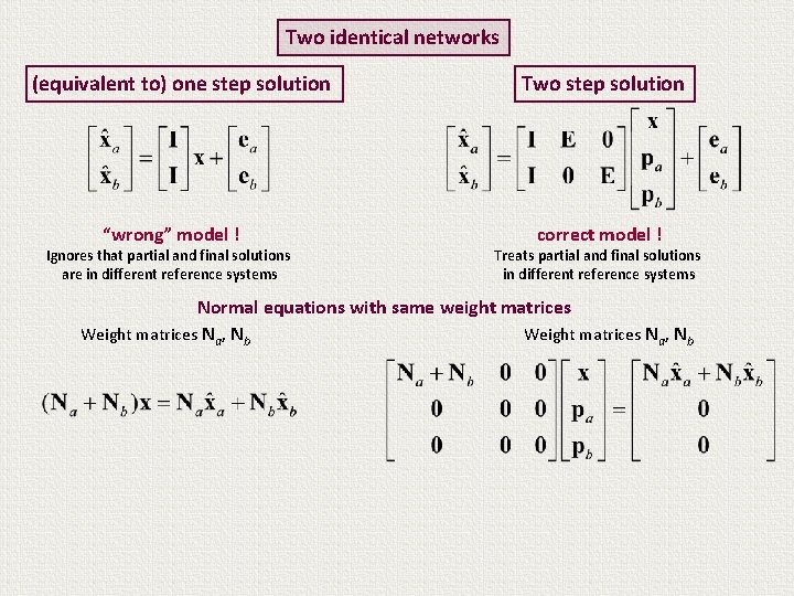
Two identical networks (equivalent to) one step solution “wrong” model ! Ignores that partial and final solutions are in different reference systems Two step solution correct model ! Treats partial and final solutions in different reference systems Normal equations with same weight matrices Weight matrices Na, Nb

Two identical networks (equivalent to) one step solution “wrong” model ! Ignores that partial and final solutions are in different reference systems Two step solution correct model ! Treats partial and final solutions in different reference systems Normal equations with same weight matrices Weight matrices Na, Nb Recall that

Two identical networks (equivalent to) one step solution Two step solution “wrong” model ! correct model ! Ignores that partial and final solutions are in different reference systems Treats partial and final solutions in different reference systems Normal equations with same weight matrices Weight matrices Na, Nb Vanishing terms

Two identical networks (equivalent to) one step solution “wrong” model ! Ignores that partial and final solutions are in different reference systems Two step solution correct model ! Treats partial and final solutions in different reference systems Normal equations with same weight matrices Weight matrices Na, Nb

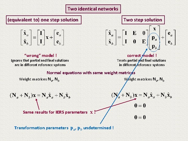
Two identical networks (equivalent to) one step solution “wrong” model ! Ignores that partial and final solutions are in different reference systems Two step solution correct model ! Treats partial and final solutions in different reference systems Normal equations with same weight matrices Weight matrices Na, Nb Same results for IERS parameters x ! Transformation parameters pa, pb undetermined !

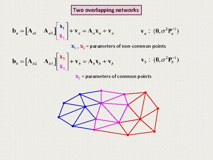
Two overlapping networks This case would apply to the ITRF formulation problem if perfect connections were available at collocation sites

Two overlapping networks x 1 , x 2 = parameters of non-common points x 3 = parameters of common points

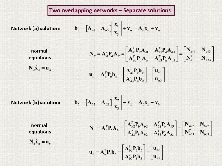
Two overlapping networks – Separate solutions Network (a) solution: normal equations Network (b) solution: normal equations

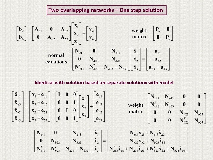
Two overlapping networks – One step solution weight matrix normal equations Identical with solution based on separate solutions with model weight matrix

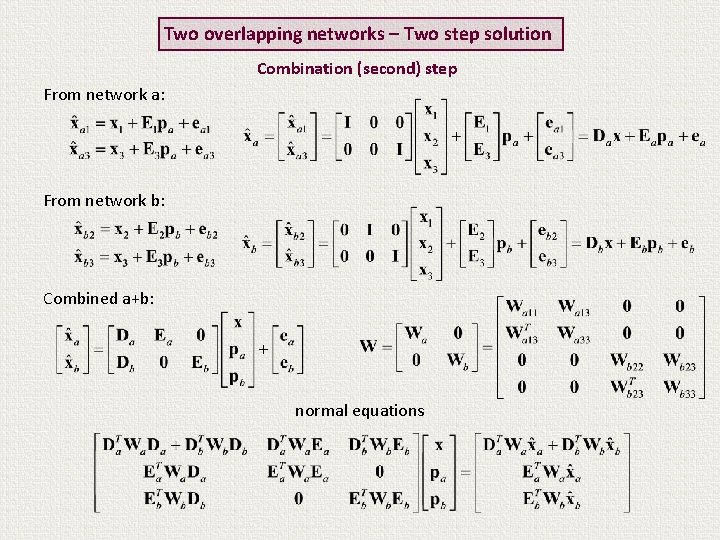
Two overlapping networks – Two step solution Combination (second) step From network a: From network b: Combined a+b: normal equations

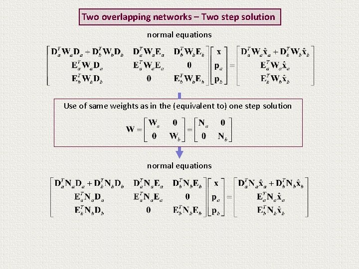
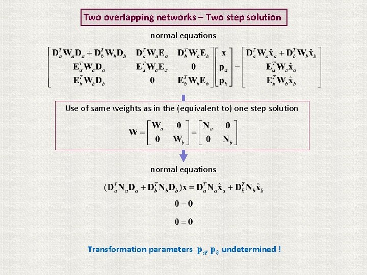
Two overlapping networks – Two step solution normal equations Use of same weights as in the (equivalent to) one step solution normal equations

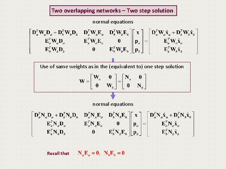
Two overlapping networks – Two step solution normal equations Use of same weights as in the (equivalent to) one step solution normal equations Recall that

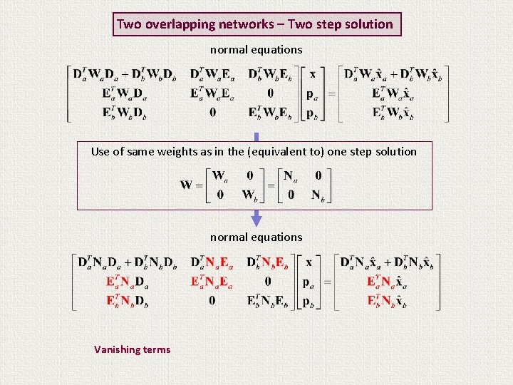
Two overlapping networks – Two step solution normal equations Use of same weights as in the (equivalent to) one step solution normal equations Vanishing terms

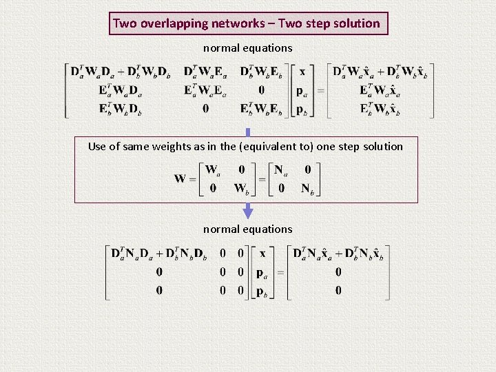
Two overlapping networks – Two step solution normal equations Use of same weights as in the (equivalent to) one step solution normal equations

Two overlapping networks – Two step solution normal equations Use of same weights as in the (equivalent to) one step solution normal equations Transformation parameters pa, pb undetermined !

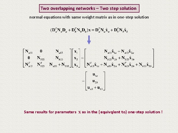
Two overlapping networks – Two step solution normal equations with same weight matrix as in one-step solution Same results for parameters x as in the (equivqlent to) one-step solution !

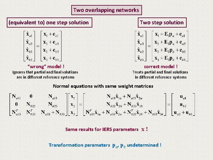
Two overlapping networks (equivalent to) one step solution “wrong” model ! Ignores that partial and final solutions are in different reference systems Two step solution correct model ! Treats partial and final solutions in different reference systems Normal equations with same weight matrices Same results for IERS parameters x ! Transformation parameters pa, pb undetermined !

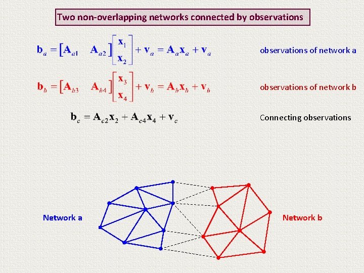
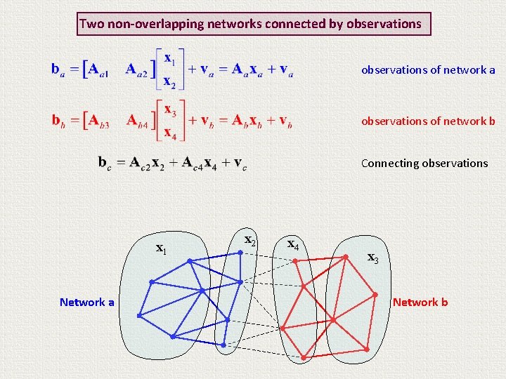
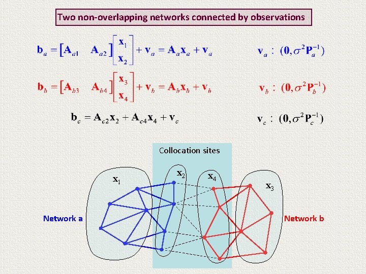
Two non-overlapping networks connected by observations This case applies to the ITRF formulation problem (with error-affected connecting observations at collocation sites)

Two non-overlapping networks connected by observations of network a observations of network b Connecting observations Network a Network b

Two non-overlapping networks connected by observations of network a observations of network b Connecting observations x 1 Network a x 2 x 4 x 3 Network b

Two non-overlapping networks connected by observations Collocation sites x 1 Network a x 2 x 4 x 3 Network b

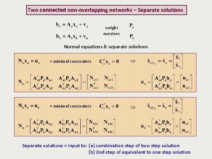
Two connected non-overlapping networks – Separate solutions weight matrices Normal equations & separate solutions + minimal constraints Separate solutions = input to: (a) combination step of two step solution (b) 2 nd step of equivalent to one step solution

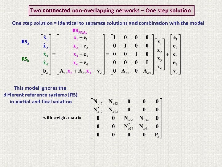
Two connected non-overlapping networks – One step solution Joint treatment of observations from network a network b & connecting observations

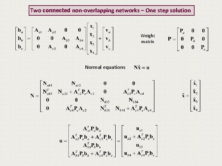
Two connected non-overlapping networks – One step solution Weight matrix Normal equations

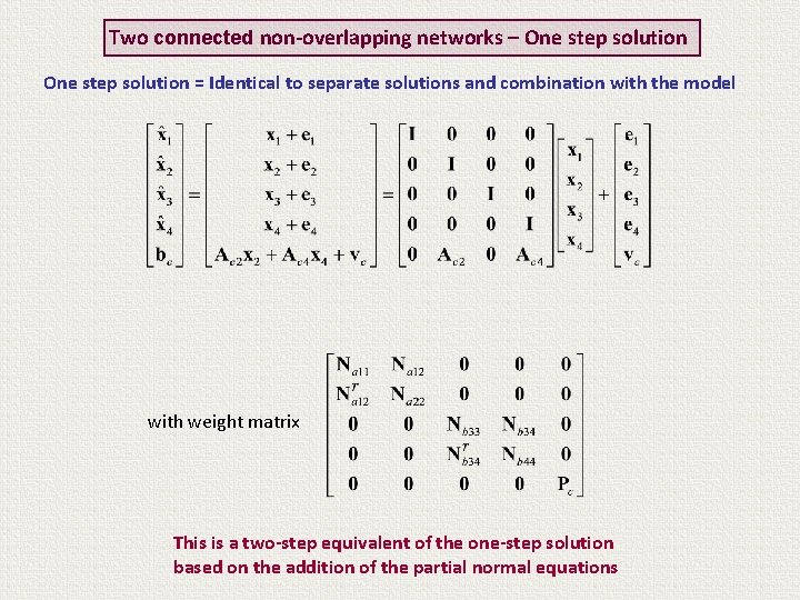
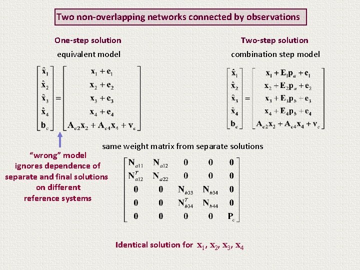
Two connected non-overlapping networks – One step solution = Identical to separate solutions and combination with the model with weight matrix This is a two-step equivalent of the one-step solution based on the addition of the partial normal equations

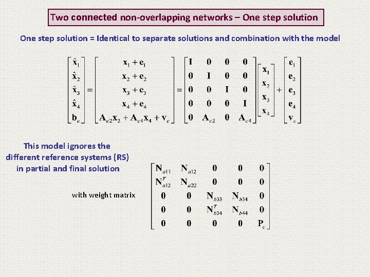
Two connected non-overlapping networks – One step solution = Identical to separate solutions and combination with the model This model ignores the different reference systems (RS) in partial and final solution with weight matrix

Two connected non-overlapping networks – One step solution = Identical to separate solutions and combination with the model RSFINAL RSa RSb This model ignores the different reference systems (RS) in partial and final solution with weight matrix

Two connected non-overlapping networks – Two step solution We have already treated the first step (separate solutions) It remains to examine the second combination step

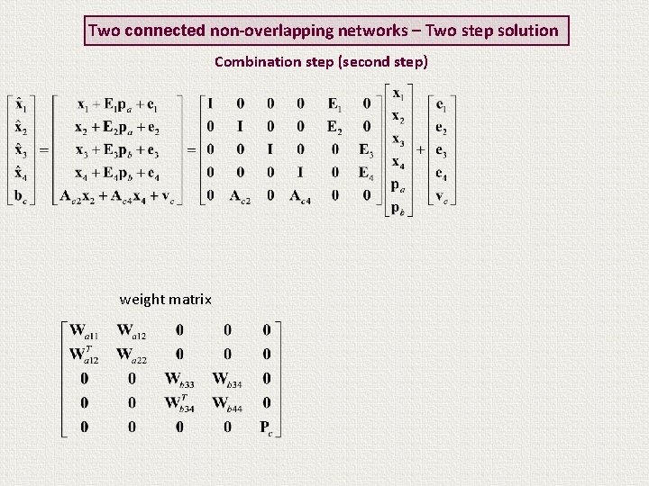
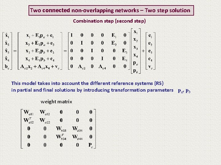
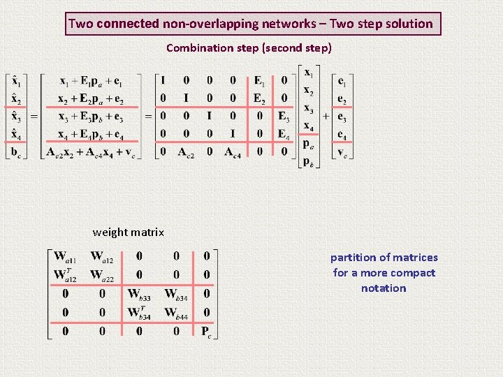
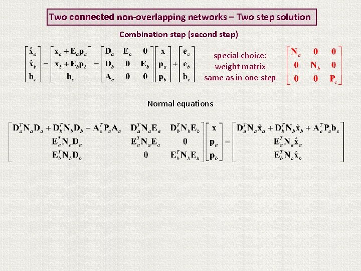
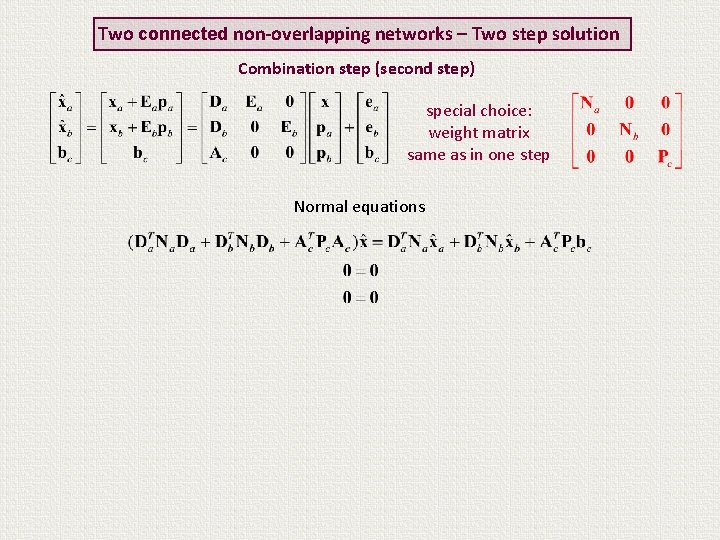
Two connected non-overlapping networks – Two step solution Combination step (second step) weight matrix

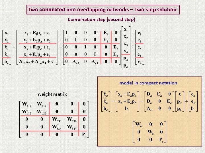
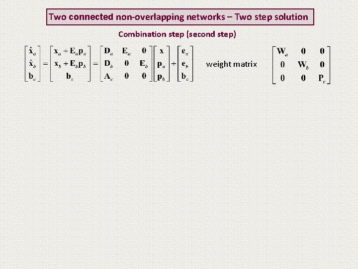
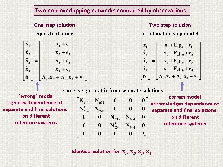
Two connected non-overlapping networks – Two step solution Combination step (second step) This model takes into account the different reference systems (RS) in partial and final solutions by introducing transformation parameters pa, pb weight matrix

Two connected non-overlapping networks – Two step solution Combination step (second step) weight matrix partition of matrices for a more compact notation

Two connected non-overlapping networks – Two step solution Combination step (second step) model in compact notation weight matrix

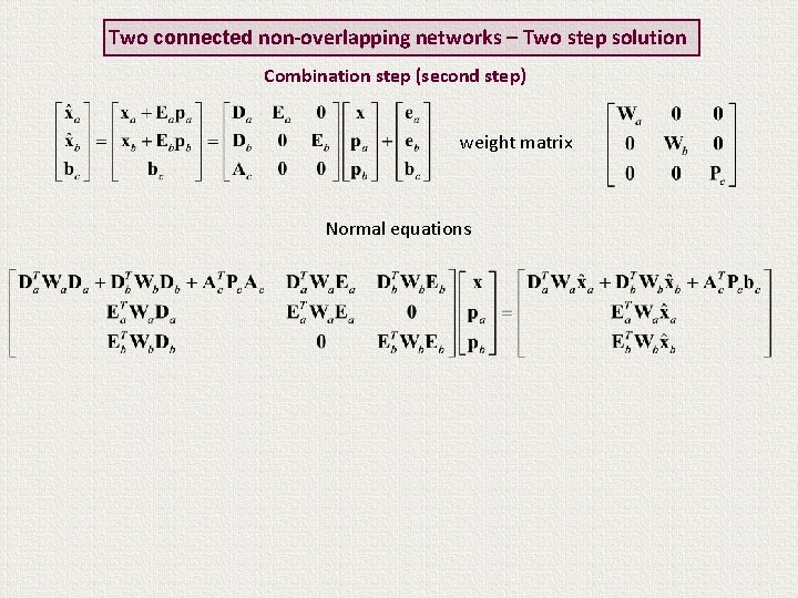
Two connected non-overlapping networks – Two step solution Combination step (second step) weight matrix

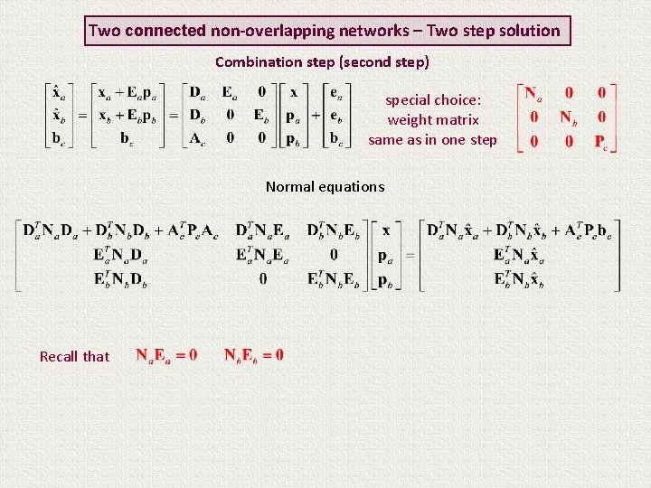
Two connected non-overlapping networks – Two step solution Combination step (second step) weight matrix Normal equations

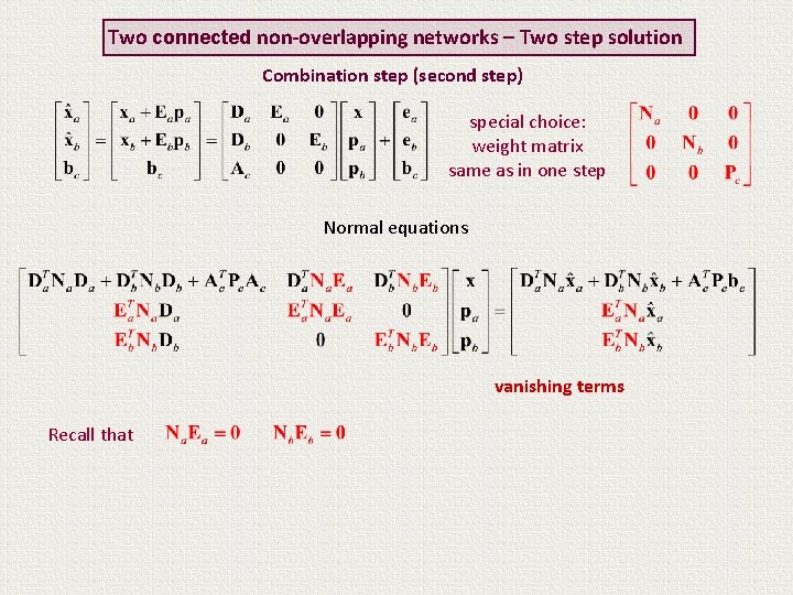
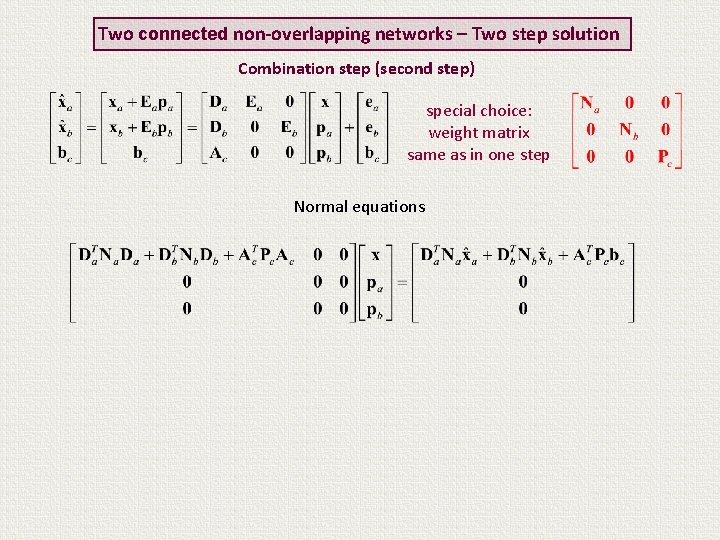
Two connected non-overlapping networks – Two step solution Combination step (second step) special choice: weight matrix same as in one step Normal equations

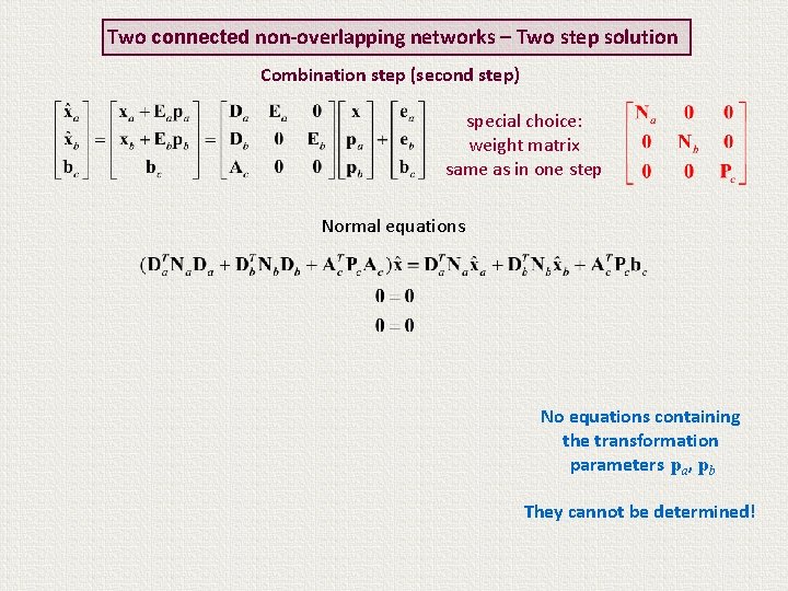
Two connected non-overlapping networks – Two step solution Combination step (second step) special choice: weight matrix same as in one step Normal equations Recall that

Two connected non-overlapping networks – Two step solution Combination step (second step) special choice: weight matrix same as in one step Normal equations vanishing terms Recall that

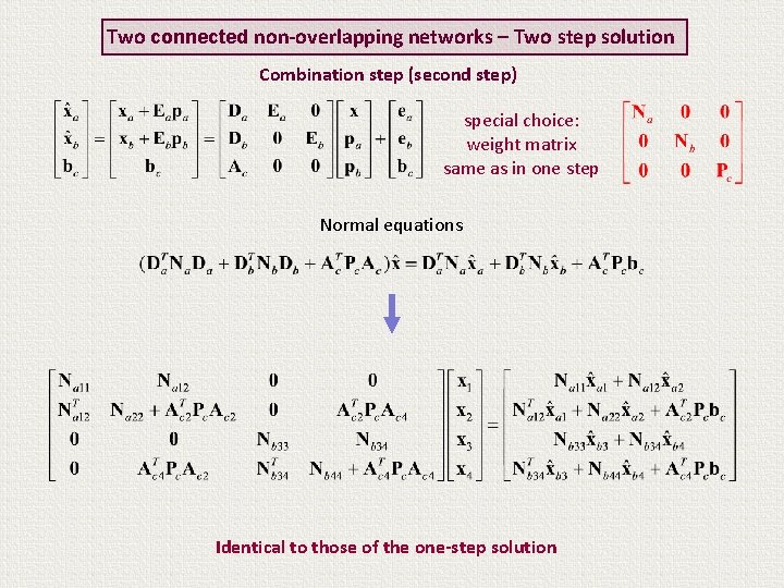
Two connected non-overlapping networks – Two step solution Combination step (second step) special choice: weight matrix same as in one step Normal equations

Two connected non-overlapping networks – Two step solution Combination step (second step) special choice: weight matrix same as in one step Normal equations

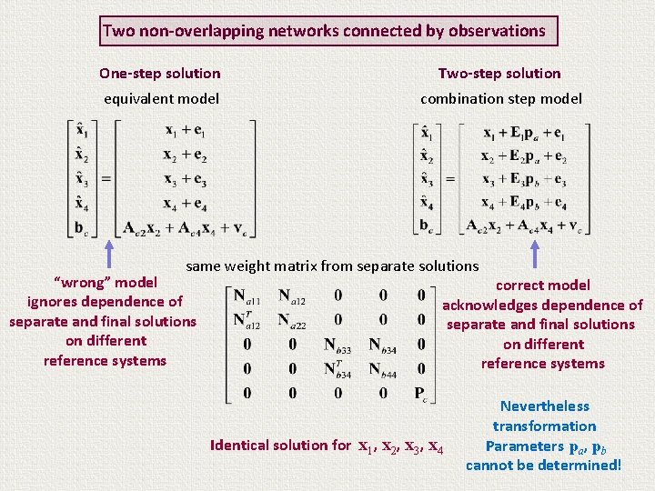
Two connected non-overlapping networks – Two step solution Combination step (second step) special choice: weight matrix same as in one step Normal equations No equations containing the transformation parameters pa, pb They cannot be determined!

Two connected non-overlapping networks – Two step solution Combination step (second step) special choice: weight matrix same as in one step Normal equations Identical to those of the one-step solution

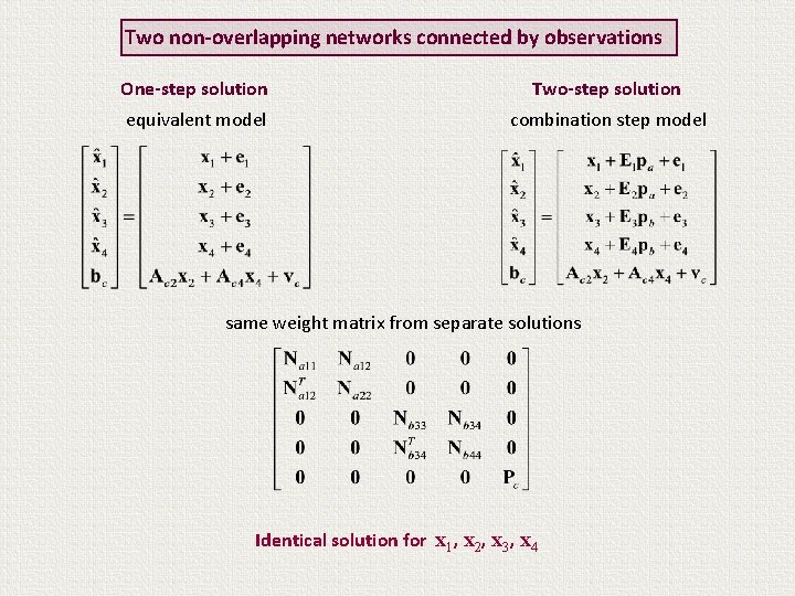
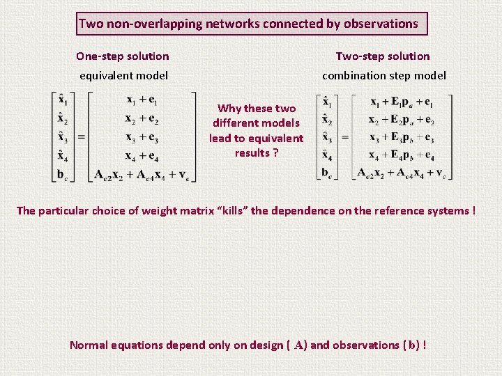
Two non-overlapping networks connected by observations One-step solution Two-step solution equivalent model combination step model same weight matrix from separate solutions Identical solution for x 1, x 2, x 3, x 4

Two non-overlapping networks connected by observations One-step solution Two-step solution equivalent model combination step model same weight matrix from separate solutions “wrong” model ignores dependence of separate and final solutions on different reference systems Identical solution for x 1, x 2, x 3, x 4

Two non-overlapping networks connected by observations One-step solution Two-step solution equivalent model combination step model same weight matrix from separate solutions “wrong” model ignores dependence of separate and final solutions on different reference systems correct model acknowledges dependence of separate and final solutions on different reference systems Identical solution for x 1, x 2, x 3, x 4

Two non-overlapping networks connected by observations One-step solution Two-step solution equivalent model combination step model same weight matrix from separate solutions “wrong” model ignores dependence of separate and final solutions on different reference systems correct model acknowledges dependence of separate and final solutions on different reference systems Identical solution for x 1, x 2, x 3, x 4 Nevertheless transformation Parameters pa, pb cannot be determined!

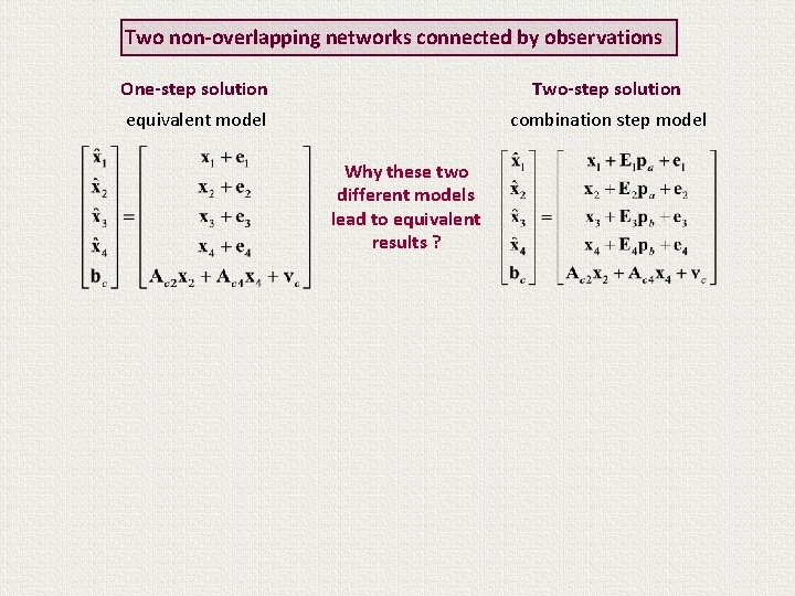
Two non-overlapping networks connected by observations One-step solution Two-step solution equivalent model combination step model Why these two different models lead to equivalent results ?

Two non-overlapping networks connected by observations One-step solution Two-step solution equivalent model combination step model Why these two different models lead to equivalent results ? The particular choice of weight matrix “kills” the dependence on the reference systems ! Normal equations depend only on design ( A) and observations ( b) !

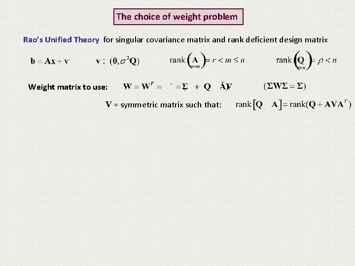
The choice of weight problem In the two step approach, the first step produces singular covariance matrices. Therefore the weight matrices to be used in the second step are not uniquely defined. This fact raises some questions about the choice of weight matrices:

The choice of weight problem In the two step approach, the first step produces singular covariance matrices. Therefore the weight matrices to be used in the second step are not uniquely defined. This fact raises some questions about the choice of weight matrices: Are the weight matrices used in order to obtain equivalent results with the one step approach the correct ones? (Do they lead to BLUUE estimates? ) Yes !

The choice of weight problem In the two step approach, the first step produces singular covariance matrices. Therefore the weight matrices to be used in the second step are not uniquely defined. This fact raises some questions about the choice of weight matrices: Are the weight matrices used in order to obtain equivalent results with the one step approach the correct ones? (Do they lead to BLUUE estimates? ) Yes ! Are there other correct weight matrices? Yes !

The choice of weight problem In the two step approach, the first step produces singular covariance matrices. Therefore the weight matrices to be used in the second step are not uniquely defined. This fact raises some questions about the choice of weight matrices: Are the weight matrices used in order to obtain equivalent results with the one step approach the correct ones? (Do they lead to BLUUE estimates? ) Yes ! Are there other correct weight matrices? Yes ! Do different correct weight matrices lead to the same results? (i. e. to estimates that are connected by a change of the reference system) Yes !

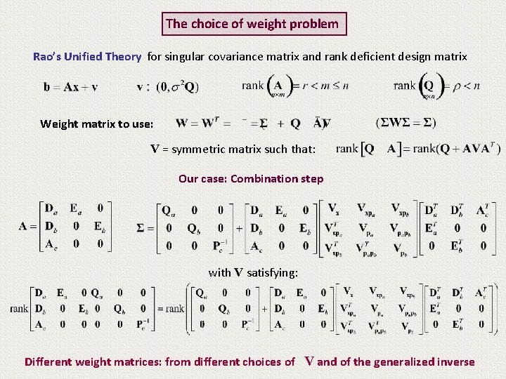
The choice of weight problem Rao’s Unified Theory for singular covariance matrix and rank deficient design matrix Weight matrix to use: V = symmetric matrix such that:

The choice of weight problem Rao’s Unified Theory for singular covariance matrix and rank deficient design matrix Weight matrix to use: V = symmetric matrix such that: Our case: Combination step with V satisfying: Different weight matrices: from different choices of V and of the generalized inverse

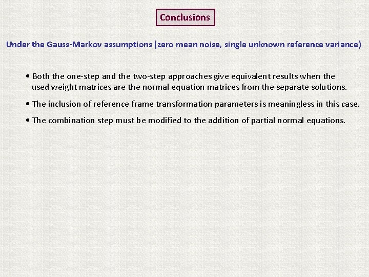
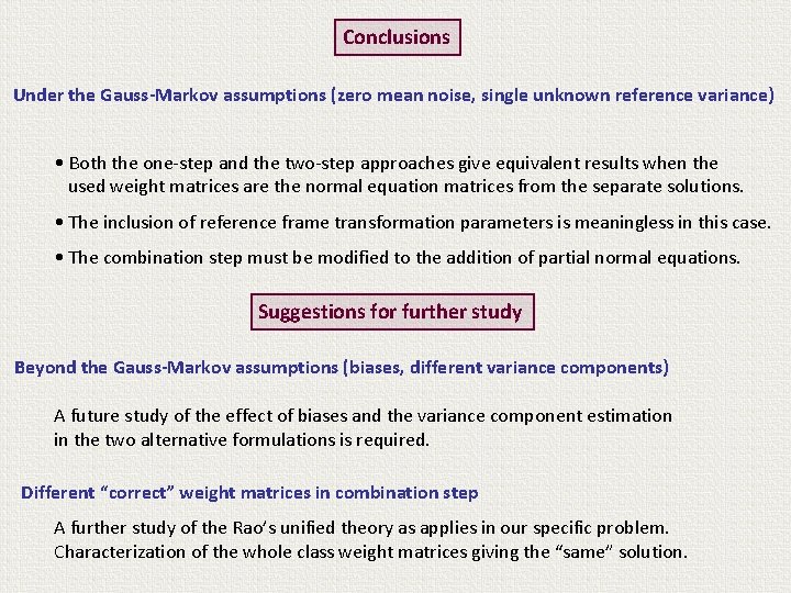
Conclusions Under the Gauss-Markov assumptions (zero mean noise, single unknown reference variance) • Both the one-step and the two-step approaches give equivalent results when the used weight matrices are the normal equation matrices from the separate solutions. • The inclusion of reference frame transformation parameters is meaningless in this case. • The combination step must be modified to the addition of partial normal equations.

Conclusions Under the Gauss-Markov assumptions (zero mean noise, single unknown reference variance) • Both the one-step and the two-step approaches give equivalent results when the used weight matrices are the normal equation matrices from the separate solutions. • The inclusion of reference frame transformation parameters is meaningless in this case. • The combination step must be modified to the addition of partial normal equations. Suggestions for further study Beyond the Gauss-Markov assumptions (biases, different variance components) A future study of the effect of biases and the variance component estimation in the two alternative formulations is required. Different “correct” weight matrices in combination step A further study of the Rao’s unified theory as applies in our specific problem. Characterization of the whole class weight matrices giving the “same” solution.

Thanks for your attention ! A copy of this presentation can be downloaded from http: //der. topo. auth. gr/