On Some Statistical Considerations in Testing for Multiple

On Some Statistical Considerations in Testing for Multiple Endpoints in Clinical Trials Mohammad Huque, Ph. D. Division of Biometrics III/Office of Biostatistics/OPa. SS/CDER/FDA ASA Biopharm Section FDA/Industry Workshop, September 21 -23, 2004, Washington, D. C. 3/9/2021

Disclaimer • The views in this presentation do not necessarily reflect those of the Food and Drug Administration 3/9/2021

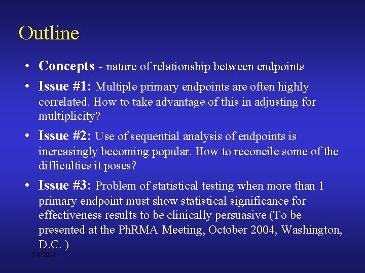
Outline • Concepts - nature of relationship between endpoints • Issue #1: Multiple primary endpoints are often highly correlated. How to take advantage of this in adjusting for multiplicity? • Issue #2: Use of sequential analysis of endpoints is increasingly becoming popular. How to reconcile some of the difficulties it poses? • Issue #3: Problem of statistical testing when more than 1 primary endpoint must show statistical significance for effectiveness results to be clinically persuasive (To be presented at the Ph. RMA Meeting, October 2004, Washington, D. C. ) 3/9/2021

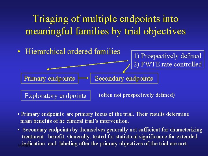
Triaging of multiple endpoints into meaningful families by trial objectives • Hierarchical ordered families Primary endpoints Exploratory endpoints 1) Prospectively defined 2) FWTE rate controlled Secondary endpoints (often not prospectively defined) • Primary endpoints are primary focus of the trial. Their results determine main benefits of he clinical trial’s intervention. • Secondary endpoints by themselves generally not sufficient for characterizing treatment benefit. Generally, tested for statistical significance for extended indication and labeling after the primary objectives of the trial are met. 3/9/2021

Nature of relationships between endpoints • Statistical independence and dependence concepts (familiar to statisticians) • Causal dependence between endpoints (related to treatment effect) Endpoint X has effect the endpoint Y will also have an effect, vice versa Examples: Diabetes trials - Hb. Ac 1 and fasting glucose levels. CHF trials – CHF related deaths and all-cause mortality. ITT versus PP endpoints • Correlation between endpoints do not necessarily imply this causal dependence (A surrogate endpoint and a clinical endpoint may be correlated w/o this property). • 3/9/2021

Extent of multiplicity adjustments between endpoints correlation high low Small adjustments Large adjustments low Practically no adjustments Good case for combining endpoints high Causal dependence (Homogeneity of treatment effects across endpoints) 3/9/2021

Issue #1: • Multiple primary endpoints are often highly correlated. How to take advantage of this in adjusting for multiplicity? 3/9/2021

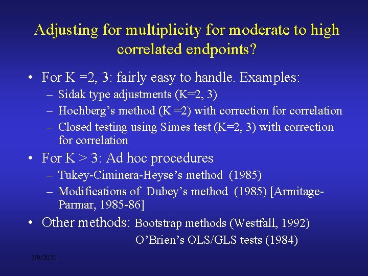
Adjusting for multiplicity for moderate to high correlated endpoints? • For K =2, 3: fairly easy to handle. Examples: – Sidak type adjustments (K=2, 3) – Hochberg’s method (K =2) with correction for correlation – Closed testing using Simes test (K=2, 3) with correction for correlation • For K > 3: Ad hoc procedures – Tukey-Ciminera-Heyse’s method (1985) – Modifications of Dubey’s method (1985) [Armitage. Parmar, 1985 -86] • Other methods: Bootstrap methods (Westfall, 1992) O’Brien’s OLS/GLS tests (1984) 3/9/2021

2 Endpoint Case: Sidak type adjustments Assumption: test statistics Z 1 and Z 2 follow bi-variate normal distribution Overall α = 0. 025, 1 -sided tests (1)Adj Corr. 2*(Adj ) 1 Adj 2 0. 01258 0. 01252 0. 00510 0. 3 0. 01292 0. 02584 0. 00559 0. 5 0. 01348 0. 02696 0. 00649 0. 7 0. 01463 0. 02926 0. 00857 0. 8 0. 01568 0. 03136 0. 01068 0. 9 0. 01751 0. 03502 0. 01464 (1) Equal adjustments for both endpoints 3/9/2021

2 Endpoint Case: Adjustment in the Hochberg method Test statistics Z 1 and Z 2 follow bi-variate normal distribution Overall αlpha = 0. 05, 2 -sided tests r Type I Adjustment Type I Test the smaller P Error rate Factor C Error Rate at level 0. 05 1 0. 05 0. 0250 0. 3 0. 04934 1. 014447 0. 05 0. 0254 0. 5 0. 04802 1. 047418 0. 05 0. 0262 0. 7 0. 04560 1. 122461 0. 05 0. 0281 0. 8 0. 04382 1. 197015 0. 0299 0. 04168 1. 335077 0. 05 0. 0334 0. 95 0. 04096 1. 470331 0. 05 0. 0368 If max (p 1, p 2) < 0. 05, then both endpoints significant If max (p 1, p 2) < 0. 05, then test the smaller p-value at level C/2 (0. 05) 3/9/2021

3 Endpoint Case: Sidak type adjustments Test statistics Z 1, Z 2 and Z 3 follow 3 -variable normal distribution Overall αlpha = 0. 025, 1 -sided tests (1)Adj (2)Adj r 12 r 13 r 23 2*(Adj ) 1 2 0 0. 00840 0. 01680 . 3. 5. 5. 5. 8 . 3. 3. 5. 5. 3 . 3. 3. 3. 5. 3 0. 00877 0. 00898 0. 00920 0. 00941 0. 00984 0. 01754 0. 01796 0. 01840 0. 01882 0. 01968 0. 00287 0. 00343 0. 00350 0. 00416 . 8. 5. 5 0. 01029 0. 01120 0. 01127 0. 01209 0. 02058 0. 02240 0. 02254 0. 02418 0. 00467 0. 00648 0. 00689 . 8. 8. 3. 8. 8. 5. 8. 8. 8 0. 02 0. 00255 (1) Equal adjustments for all 3 endpoints (2) alpha 1= 0. 02 for the 1 st endpoint and adjusted alpha 2= adjusted alpha 3 3/9/2021

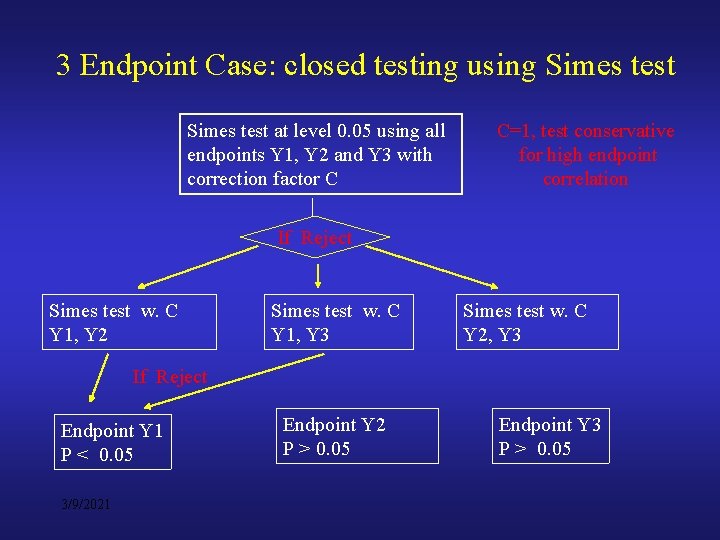
3 Endpoint Case: closed testing using Simes test at level 0. 05 using all endpoints Y 1, Y 2 and Y 3 with correction factor C C=1, test conservative for high endpoint correlation If Reject Simes test w. C Y 1, Y 2 Simes test w. C Y 1, Y 3 Simes test w. C Y 2, Y 3 If Reject Endpoint Y 1 P < 0. 05 3/9/2021 Endpoint Y 2 P > 0. 05 Endpoint Y 3 P > 0. 05

Correction factor C for the Simes test, K=3 Test statistics Z 1, Z 2 and Z 3 follow 3 -variable normal distribution αlpha = 0. 05, 2 -sided tests r Type I Adjustment Type I Error rate Factor C Error Rate 0. 05 1 0. 05 0. 3 0. 0489 1. 02200 0. 05 0. 0468 1. 07202 0. 05 0. 7 0. 0430 1. 17916 0. 05 0. 8 0. 0403 1. 27227 0. 05 0. 9 0. 0374 1. 40980 0. 05 Effectiveness in at least one endpoint, if p(3) < 0. 05, or { P(3) 0. 05, P(2) < 0. 05*2/3*C}, or { P(3) 0. 05, P(2) 0. 05*2/3*C, P(1) <. 05*1/3*C}. 3/9/2021

Case of Dependent Event Rate Endpoints Dependence parameter can be estimated as follows: Y= hospitalization endpoint X= mortality endpoint x=1, y =1 p 11 x=0, y =1 p 01 p’ x=1, y =0 p 10 x=0, y =0 p 00 q’ p q Dependence parameter = p 11/ (pqp’q’) • Approximate test statistics for the proportions are bivariate normal in the limit with the above dependence parameter 3/9/2021 • Previous methods for the continuous endpoints apply

TCH (Tukey-Ciminera-Heyse, 1985) and Dubey (1985) tests (K >3) • TCH method (highly correlated endpoints, 1985) Adjusted alpha = 1 - (1 -alpha) 1/sqrt (K) • Dubey (1985) [Armitage-Parmar (1985 -86)] Adjusted alpha = 1 - (1 -alpha) 1/mi m = K (1 - r. i), (i = 1, …, K), i r. i = average of (K-1) correlation coefficients (ith endpoint vs. the other K-1 endpoints) • Recent modifications of the Dubey method for proper protection of the type I error rate 3/9/2021

Modifications of the Dubey’s method First step - correlation matrix conversion • Convert correlation rij to corr ( (|Zi|, (|Zj|), Zi and Zj follow standard 2 -variable normal distribution w. correlation coefficient rij r = (0. 1, 0. 2, 0. 3, 0. 4, 0. 5, 0. 6, 0. 7, 0. 8, 0. 9) converts to (0. 00609, 0. 02264, 0. 05641, 0. 10282, 0. 16608, 0. 24980, 0. 35936, 0. 50400, 0. 70109) 3/9/2021

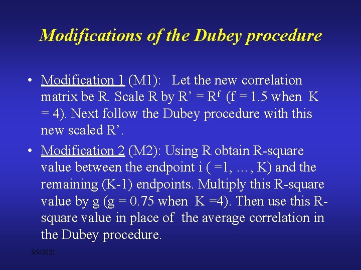
Modifications of the Dubey procedure • Modification 1 (M 1): Let the new correlation matrix be R. Scale R by R’ = Rf (f = 1. 5 when K = 4). Next follow the Dubey procedure with this new scaled R’. • Modification 2 (M 2): Using R obtain R-square value between the endpoint i ( =1, …, K) and the remaining (K-1) endpoints. Multiply this R-square value by g (g = 0. 75 when K =4). Then use this Rsquare value in place of the average correlation in the Dubey procedure. 3/9/2021

Performance of the ad hoc procedures for K=4 for some correlation structures R = {r 12, r 13, r 14, r 23, r 24, r 34} R 1 = {. 9 (3), . 8 (2), . 3 } all v. high -one low (Avg 7. 7) R 2 = {. 8 (2), . 5(2), . 3 (2) } 2 v. high, 2 medium, 2 low (5. 3) R 3 = {. 7 (3), . 5(2), . 1 } 3 high, 2 medium, 1 v. low ( 5. 3) R 4 = {. 8, . 7, . 3 (2), . 1 (2)} 1 v. high, 1 high, 2 low, 1 v. low ( 3. 7) R 5 = {. 8 , . 5, . 3, . 1 (3)} 1 high, 1 medium, 1 low, 1 v. low (3. 2) R 6 = {. 5 (2), . 4, . 3 (2), . 1} 3 medium, 2 low, 1 v. low ( 3. 5) R 7 = (. 5(2), . 4, . 1 (3)} 3 medium, 3 v. low ( 2. 8) R 8 = (. 2 (3). . 1 (3)} all v. low ( 1. 5) 3/9/2021

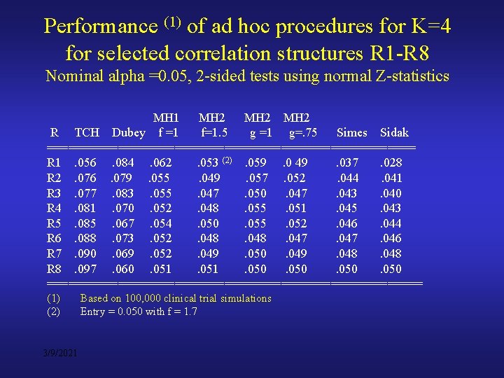
Performance (1) of ad hoc procedures for K=4 for selected correlation structures R 1 -R 8 Nominal alpha =0. 05, 2 -sided tests using normal Z-statistics MH 1 MH 2 R TCH Dubey f =1 f=1. 5 g =1 g=. 75 Simes Sidak ========================== R 1. 056. 084. 062. 053 (2). 059. 0 49. 037. 028 R 2. 076. 079. 055. 049. 057. 052. 044. 041 R 3. 077. 083. 055. 047. 050. 047. 043. 040 R 4. 081. 070. 052. 048. 055. 051. 045. 043 R 5. 085. 067. 054. 050. 055. 052. 046. 044 R 6. 088. 073. 052. 048. 047. 046 R 7. 090. 069. 052. 049. 050. 049. 048 R 8. 097. 060. 051. 050 =========================== (1) (2) 3/9/2021 Based on 100, 000 clinical trial simulations Entry = 0. 050 with f = 1. 7

Some comments on the results of the previous table • Investigations limited to selected correlation structures for K =4 • Tukey’s adjustment – for highly correlated endpoints • Dubey’s – fairly stable, but liberal in protecting alpha-level • Mofication M 2 (g =. 75) performs well • The approach sensitive to the choice of metric and scaling factor • Simes and Sidak methods quite conservative for moderate to high correlated endpoints 3/9/2021

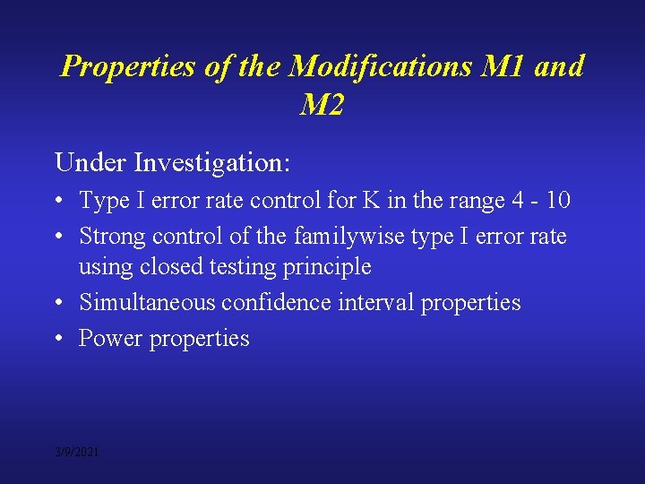
Properties of the Modifications M 1 and M 2 Under Investigation: • Type I error rate control for K in the range 4 - 10 • Strong control of the familywise type I error rate using closed testing principle • Simultaneous confidence interval properties • Power properties 3/9/2021

O’Brien’s OLS/GLS t-tests, 1984 (K > 3) These tests are based on weighted sums of the K standardized endpoints using weights (w 1, w 2, …, w. K) = JT R-1 for the GLS test and = JT for the OLS test. In other words, GLS method give more weights to endpoints not highly correlated and the OLS method gives equal weight to all endpoints. • Test sensitive under homogeneity of treatment effects and low correlation across endpoints • Performs poorly under treatment by endpoint interaction • Closed testing for endpoint specific results 3/9/2021

Issue #2 • Use of sequential analysis of endpoints is increasingly becoming popular. How to reconcile some of the difficulties it poses? Suppose that the sequence breaks, and the subsequent endpoint has an extremely low value. How avoid this situation? 3/9/2021

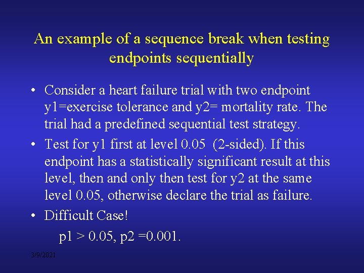
An example of a sequence break when testing endpoints sequentially • Consider a heart failure trial with two endpoint y 1=exercise tolerance and y 2= mortality rate. The trial had a predefined sequential test strategy. • Test for y 1 first at level 0. 05 (2 -sided). If this endpoint has a statistically significant result at this level, then and only then test for y 2 at the same level 0. 05, otherwise declare the trial as failure. • Difficult Case! p 1 > 0. 05, p 2 =0. 001. 3/9/2021

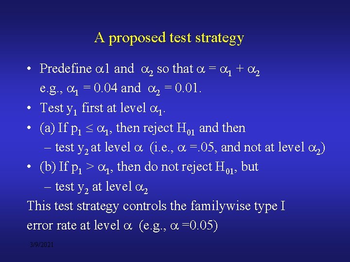
A proposed test strategy • Predefine 1 and 2 so that = 1 + 2 e. g. , 1 = 0. 04 and 2 = 0. 01. • Test y 1 first at level 1. • (a) If p 1 1, then reject H 01 and then – test y 2 at level (i. e. , =. 05, and not at level 2) • (b) If p 1 > 1, then do not reject H 01, but – test y 2 at level 2 This test strategy controls the familywise type I error rate at level (e. g. , =0. 05) 3/9/2021

Concluding Remarks • Understanding of relationships between endpoints helps in selecting an efficient test strategy for multiple endpoints • Methods that account for correlation between endpoints are fairly straightforward for K=2, 3 • Ad hoc procedures such as M 1 and M 2 modifications of the Dubey’s procedure can be helpful in testing for K > 3. Also bootstrap and O’Brien’s methods can be applied • Sequential testing can be done slightly differently to accommodate sequence breaks with extreme subsequent p-values 3/9/2021