On Lattices Learning with Errors Random Linear Codes

On Lattices, Learning with Errors, Random Linear Codes, and Cryptography Oded Regev Tel-Aviv University

Outline • Introduction to lattices • Main theorem: a hard learning problem • Application: a stronger and more efficient public key cryptosystem • Proof of main theorem • Overview • Part I: Quantum • Part II: Classical

Lattices Basis: v 1, …, vn vectors in Rn The lattice L is 2 v 1 v 1+v 2 L={a 1 v 1+…+anvn| ai integers} The dual lattice of L is L*={x | 8 y 2 L, hx, yi 2 Z} v 1 2 v 2 -v 1 2 v 2 -2 v 1 0

Shortest Vector Problem (SVP) v 2 v 1 0 • SVP: Given a lattice, find an approximately shortest vector

Closest Vector Problem (CVPd) v 0 • CVPd: Given a lattice and a target vector within distance d, find the closest lattice point

Main Theorem Hardness of Learning

Learning from parity with error • Let s 2 Z 2 n be a secret • We have random equations modulo 2 with error (everything independent): s 2+s 3+s 4+ s 6+…+sn 0 s 1+s 2+ s 4+ s 6+…+sn 1 s 1+ s 3+s 4+s 5+ …+sn 1 s 2+s 3+s 4+ s 6+…+sn 0. . . • Without error, it’s easy!

Learning from parity with error • More formally, we need to learn s from samples of the form (t, st+e) where t is chosen uniformly from Z 2 n and e is a bit that is 1 with probability 10%. • Easy algorithms need 2 O(n) equations/time • Best algorithm needs 2 O(n/logn) equations/time [Blum. Kalai. Wasserman’ 00] • Open question: why is this problem so hard?

Learning modulo p • Fix some p<poly(n) • Let s 2 Zpn be a secret • We have random equations modulo p with error: 2 s 1+0 s 2+2 s 3+1 s 4+2 s 5+4 s 6+…+4 sn 0 s 1+1 s 2+5 s 3+0 s 4+6 s 5+6 s 6+…+2 sn 6 s 1+5 s 2+2 s 3+0 s 4+5 s 5+2 s 6+…+0 sn 6 s 1+4 s 2+4 s 3+4 s 4+3 s 5+3 s 6+…+1 sn. . . 2 4 2 5

Learning modulo p • More formally, we need to learn s from samples of the form (t, st+e) where t is chosen uniformly from Zpn and e is chosen from Zp • Easy algorithms need 2 O(nlogn) equations/time • Best algorithm needs 2 O(n) equations/time [Blum. Kalai. Wasserman’ 00]

Main Theorem Learning modulo p is as hard as worst-case lattice problems using a quantum reduction • In other words: solving the problem implies an efficient quantum algorithm for lattices

Equivalent formulation • For m=poly(n), let C be a random m£n matrix • with elements in Zp. Given Cs+e for some s Zpn and some noise vector e Zpm, recover s. This is the problem of decoding from a random linear code

Why Quantum? • As part of the reduction, we need to • perform a certain algorithmic task on lattices We do not know how to do it classically, only quantumly!

Why Quantum? • • x y We are given an oracle that solves CVPd for some small d As far as I can see, the only way to generate inputs to this oracle is: • Somehow choose x L • Let y be some random vector within dist d of x • Call the oracle with y The answer is x. But we already know the answer !! Quantumly, being able to compute x from y is very useful: it allows us to transform the state |y, x> to the state |y, 0> reversibly (and then we can apply the quantum Fourier transform)

Application: New Public Key Encryption Scheme

Previous lattice-based PKES [Ajtai. Dwork 96, Goldreich. Goldwasser. Halevi 97, R’ 03] • Main advantages: • Based on a lattice problem • Worst-case hardness • Main disadvantages: • Based only on unique-SVP • Impractical (think of n as 100): • Public key size O(n 4) • Encryption expands by O(n 2)

Ajtai’s recent PKES [Ajtai 05] • Main advantages: • Practical (think of n as 100): • Public key size O(n) • Encryption expands by O(n) • Main disadvantages: • Not based on lattice problem • No worst-case hardness

New lattice-based PKES [This work] • Main advantages: quantum • • • Worst-case hardness • Based on the main lattice problems (SVP, SIVP) • Practical (think of n as 100): • Public key size O(n) • Encryption expands by O(n) Breaking the cryptosystem implies an efficient quantum algorithm for lattices In fact, security is based on the learning problem (no quantum needed here)

• • • The Cryptosystem Everything modulo 4 Private key: 4 random numbers 1 2 0 3 Public key: a 6 x 4 matrix and approximate inner product 2· 1 ? + 0 · 2 ? + 1 · 0 ? + 2 · 3 ? = ≈ 0 1 1· 1 ? + 2 · 2 ? + 2 · 0 ? + 3 · 3 ? = ≈ 2 0· 1 ? + 2 · 2 ? + 0 · 0 ? + 3 · 3 ? = ≈ 1 1· 1 ? + 2 · 2 ? + 0 · 0 ? + 2 · 3 ? = ≈ 3 0 0· 1 ? + 3 · 2 ? + 1 · 0 ? + 3 · 3 ? = ≈ 3 3· 1 ? + 3 · 2 ? + 0 · 0 ? + 2 · 3 ? = ≈ 3 2 Encrypt the bit 0: 3·? + 2 ·? + 1 ·? + 0 ·? ≈ 1 Encrypt the bit 1: 3·? + 2 ·? + 1 ·? + 0 ·? ≈ 3

Proof of the Main Theorem Overview

Gaussian Distribution • Define a Gaussian distribution on a lattice (normalization omitted) • We can efficiently sample from Dr for large r=2 n

The Reduction • Assume the existence of an algorithm for the learning modulo p problem for p=2√n • Our lattice algorithm: • r=2 n • Take poly(n) samples from Dr • Repeat: • Given poly(n) samples from Dr compute poly(n) samples from Dr/2 • Set r←r/2 • When r is small, output a short vector

Dr

Dr/2

Obtaining Dr/2 from Dr • Lemma 1: p=2√n Given poly(n) samples from Dr, and an oracle for ‘learning modulo p’, we can solve CVPp/r in L* • No quantum here • Lemma 2: Given a solution to CVPd in L*, we can obtain samples from D√n/d • Quantum • Based on the quantum Fourier transform

Classical, uses learning oracle Quantum Samples from Dr in L Solution to CVPp/r in L* Samples from Dr/2 in L Solution to CVP 2 p/r in L* Samples from Dr/4 in L Solution to CVP 4 p/r in L*

Fourier Transform Primal world (L) Dual world (L*)

Fourier Transform • The Fourier transform of Dr is given by • Its value is • 1 for x in L*, • e-1 at points of distance 1/r from L*, • ¼ 0 at points far away from L*.

Proof of the Main Theorem Lemma 2: Obtaining D√n/d from CVPd

From CVPd to D√n/d • Assume we can solve CVPd; we’ll show to obtain samples from D√n/d • Step 1: Create the quantum state by adding a Gaussian to each lattice point and uncomputing the lattice point by using the CVP algorithm

• Step 2: From CVPd to D√n/d Compute the quantum Fourier transform of It is exactly D√n/d !! • Step 3: Measure and obtain one sample from D√n/d • By repeating this process, we can obtain poly(n) samples

From CVPd to D√n/d • More precisely, create the state • And the state • Tensor them together and add first to second • Uncompute first register by solving CVPp/r

Proof of the Main Theorem Lemma 1: Solving CVPp/r given samples from Dr and an oracle for learning mod p

It’s enough to approximate fp/r • Lemma: being able to approximate fp/r implies a solution to CVPp/r • Proof Idea – walk uphill: • fp/r(x)>¼ for points x of distance < p/r • Keep making small modifications to x as long as fp/r(x) increases • Stop when fp/r(x)=1 (then we are on a lattice point)

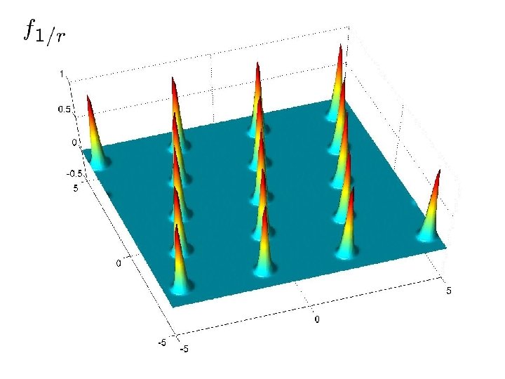
What’s ahead in this part • For warm-up, we show to approximate f 1/r given samples from Dr • No need for learning • This is main idea in [Aharonov. R’ 04] • Then we show to approximate f 2/r given samples from Dr and an oracle for the learning problem • Approximating fp/r is similar

Warm-up: approximating f 1/r • Let’s write f 1/r in its Fourier representation: • Using samples from Dr, we can compute a good approximation to f 1/r (this is the main idea in [Aharonov. R’ 04])

Fourier Transform • Consider the Fourier representation again: • For x 2 L*, hw, xi is integer for all w in L and • therefore we get f 1/r(x)=1 For x that is close to L*, hw, xi is distributed around an integer. Its standard deviation can be (say) 1.

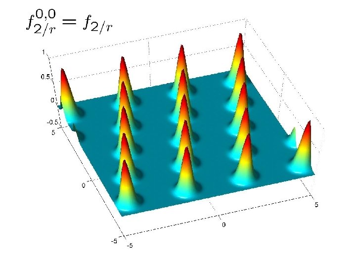
Approximating f 2/r • Main idea: partition Dr into 2 n distributions • For t (Z 2)n, denote the translate t by Dtr • Given a lattice point we can compute its t • The probability on (Z 2)n obtained by sampling from Dr and outputting t is close to uniform 0, 0 0, 1 1, 0 1, 1

Approximating f 2/r • Hence, by using samples from Dr we can produce samples from the following distribution on pairs (t, w): • Sample t (Z 2)n uniformly at random • Sample w from Dtr • Consider the Fourier transform of Dtr

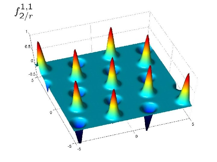
Approximating f 2/r • The functions ft 2/r look almost like f 2/r • Only difference is that some Gaussians have their • • sign flipped Approximating ft 2/r is enough: we can easily take the absolute value and obtain f 2/r For this, however, we need to obtain several pairs (t, w) for the same t • The problem is that each sample (t, w) has a different t !

Approximating f 2/r • Fix x close to L* • The sign of its Gaussian is ± 1 depending on hs, ti mod • • 2 for s (Z 2)n that depends only on x The distribution of x, w mod 2 when w is sampled from Dtr is centred around s, t mod 2 Hence, we obtain equations modulo 2 with error: hs, t 1 i ¼dhx, w 1 ic mod 2 hs, t 2 i ¼dhx, w 2 ic mod 2 hs, t 3 i ¼dhx, w 3 ic mod 2. . .

Approximating f 2/r • Using the learning algorithm, we solve these equations and obtain s • Knowing s, we cancel the sign • Averaging over enough samples gives us an approximation to f 2/r

Open Problems 1/4 • Dequantize the reduction: • This would lead to the ‘ultimate’ lattice- based cryptosystem (based on SVP, efficient) • Main obstacle: what can one do classically with a solution to CVPd? • Construct even more efficient schemes based on special classes of lattices such as cyclic lattices • For hash functions this was done by Micciancio

Open Problems 2/4 • Extend to learning from parity (i. e. , p=2) or even some constant p • Is there something inherently different about the case of constant p? • Use the ‘learning mod p’ problem to derive other lattice-based hardness results • Recently, used by Klivans and Sherstov to derive hardness of learning problems

Open Problems 3/4 • Cryptanalysis • Current attacks limited to low dimension [Nguyen. Stern 98] • New systems [Ajtai 05, R 05] are efficient and can be easily used with dimension 100+ • Security against chosen-ciphertext attacks • Known lattice-based cryptosystems are not secure against CCA

Open Problems 4/4 • Comparison with number theoretic cryptography • E. g. , can one factor integers using an oracle for n-approximate SVP? • Signature schemes • Can one construct provably secure latticebased signature schemes?