ON EFFICIENT SPATIAL MATCHING RAYMOND CHIWING WONG THE

ON EFFICIENT SPATIAL MATCHING RAYMOND CHI-WING WONG (THE CHINESE UNIVERSITY OF HONG KONG) YUFEI TAO (THE CHINESE UNIVERSITY OF HONG KONG) ADA WAI-CHEE FU (THE CHINESE UNIVERSITY OF HONG KONG) XIAOKUI XIAO (THE CHINESE UNIVERSITY OF HONG KONG) Presented by: Chan Kit Yan, Anissa Chau Chun Wai, Vincent Chau Ming Lung, Aaron Tse Wai Lam, Forest

OUTLINE Introduction � Bichromatic Reverse Nearest Neighbor (BRNN) Problem � Spatial Matching Problem (SPM) Unweighted SPM Weighted SPM Related Work Closest Pair � Stable Marriage � Algorithm Chain for Unweighted SPM � Chain for Wighted SPM � Empirical Study Conclusion

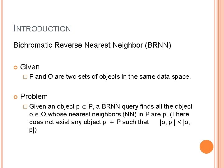
INTRODUCTION Bichromatic Reverse Nearest Neighbor (BRNN) Given �P and O are two sets of objects in the same data space. Problem an object p P, a BRNN query finds all the object o O whose nearest neighbors (NN) in P are p. (There does not exist any object p’ P such that |o, p’| < |o, p|) � Given

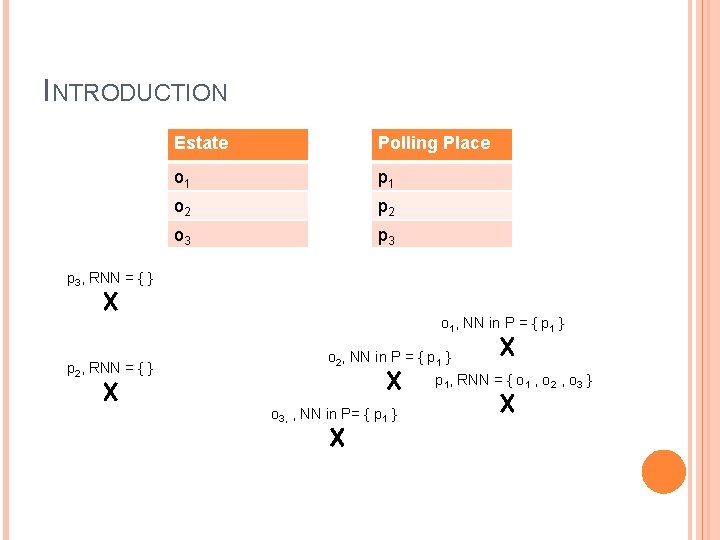
INTRODUCTION Estate Polling Place o 1 p 1 o 2 p 2 o 3 p 3, RNN = { } o 1, NN in P = { p 1 } p 2, RNN = { } o 2, NN in P = { p 1 } p 1, RNN = { o 1 , o 2 , o 3 } o 3, , NN in P= { p 1 }

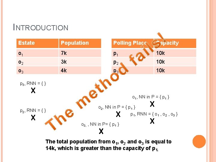
INTRODUCTION Estate Population Polling Place Capacity o 1 7 k p 1 10 k o 2 3 k p 2 10 k o 3 4 k p 3 10 k p 3, RNN = { } o 1, NN in P = { p 1 } p 2, RNN = { } o 2, NN in P = { p 1 } p 1, RNN = { o 1 , o 2 , o 3 } o 3, , NN in P= { p 1 } The total population from o 1, o 2 and o 3 is equal to 14 k, which is greater than the capacity of p 1.

INTRODUCTION Our Goal � Allocate each estate o O to the polling-place p P that (i) is as near to o as possible, and (ii) its servicing capacity has not been exhausted in serving other closer estates.

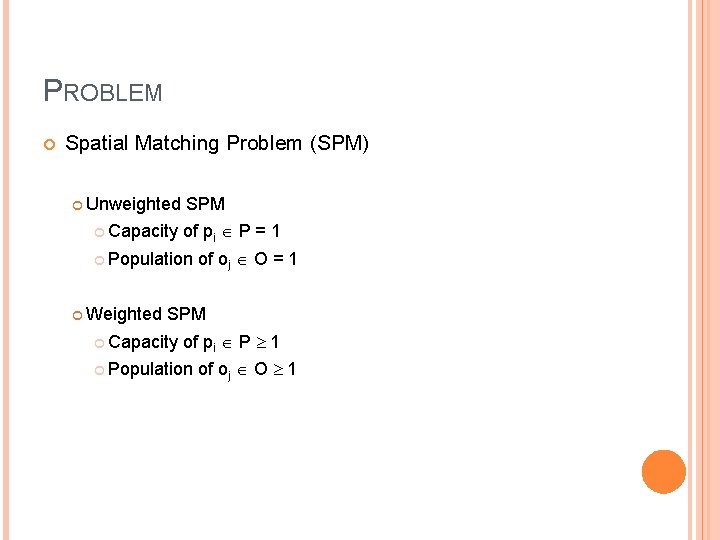
PROBLEM Spatial Matching Problem (SPM) Unweighted Capacity SPM of pi P = 1 Population Weighted of oj O = 1 SPM Capacity of pi P 1 Population of oj O 1

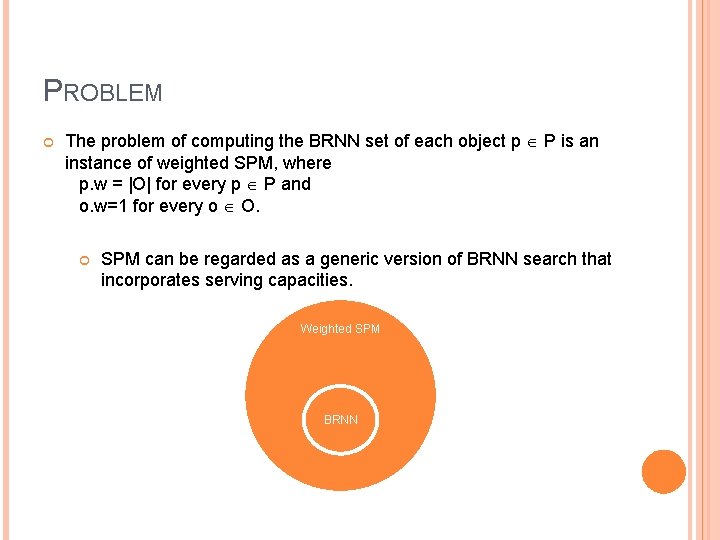
PROBLEM The problem of computing the BRNN set of each object p P is an instance of weighted SPM, where p. w = |O| for every p P and o. w=1 for every o O. SPM can be regarded as a generic version of BRNN search that incorporates serving capacities. Weighted SPM BRNN

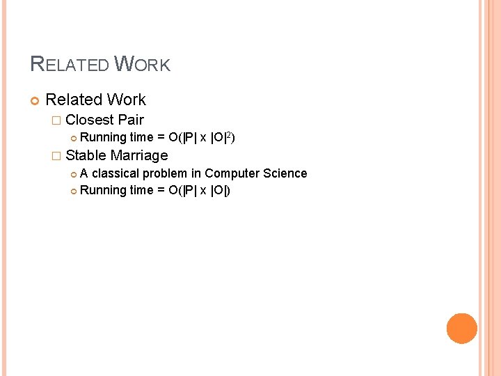
RELATED WORK Related Work � Closest Pair Running time = O(|P| x |O|2) � Stable Marriage A classical problem in Computer Science Running time = O(|P| x |O|)

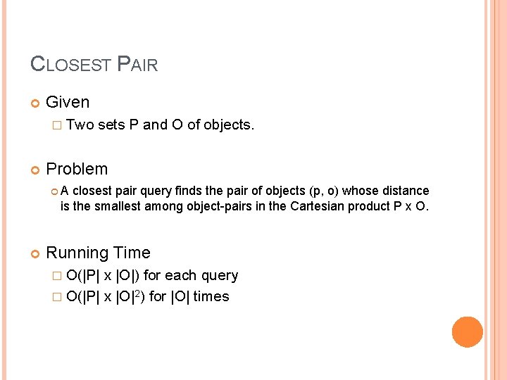
CLOSEST PAIR Given � Two sets P and O of objects. Problem A closest pair query finds the pair of objects (p, o) whose distance is the smallest among object-pairs in the Cartesian product P x O. Running Time � O(|P| x |O|) for each query � O(|P| x |O|2) for |O| times

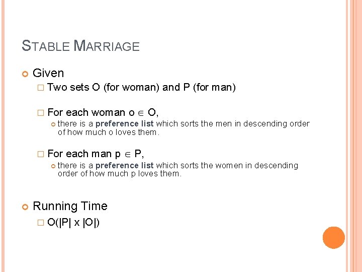
STABLE MARRIAGE Given � Two sets O (for woman) and P (for man) � For each woman o O, there is a preference list which sorts the men in descending order of how much o loves them. � For each man p P, there is a preference list which sorts the women in descending order of how much p loves them. Running Time � O(|P| x |O|)

ALGORITHM Algorithm � Chain for Unweighted/Weighted SPM - Fairness Result - High Efficiency

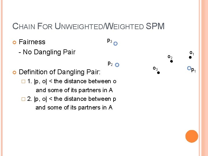
CHAIN FOR UNWEIGHTED/WEIGHTED SPM Fairness - No Dangling Pair p 3 p 2 Definition of Dangling Pair: � 1. |p, o| < the distance between o and some of its partners in A � 2. |p, o| < the distance between p and some of its partners in A o 2 o 3 o 1 p 1

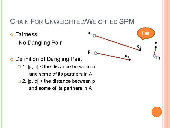
CHAIN FOR UNWEIGHTED/WEIGHTED SPM Fairness - No Dangling Pair p 3 p 2 Definition of Dangling Pair: � 1. |p, o| < the distance between o and some of its partners in A � 2. |p, o| < the distance between p and some of its partners in A Fair o 2 o 3 o 1 p 1

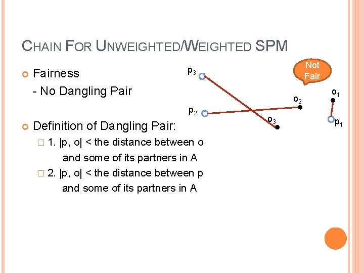
CHAIN FOR UNWEIGHTED/WEIGHTED SPM Fairness - No Dangling Pair p 2 Definition of Dangling Pair: � 1. Not Fair p 3 |p, o| < the distance between o and some of its partners in A � 2. |p, o| < the distance between p and some of its partners in A o 2 o 3 o 1 p 1

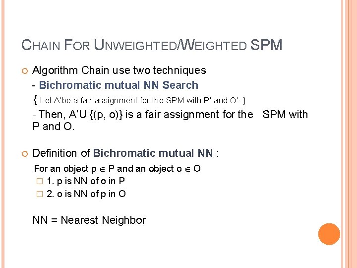
CHAIN FOR UNWEIGHTED/WEIGHTED SPM Algorithm Chain use two techniques - Bichromatic mutual NN Search { Let A’be a fair assignment for the SPM with P’ and O’. } - Then, A’U {(p, o)} is a fair assignment for the SPM with P and O. Definition of Bichromatic mutual NN : For an object p P and an object o O � 1. p is NN of o in P � 2. o is NN of p in O NN = Nearest Neighbor

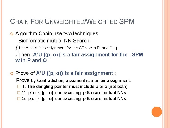
CHAIN FOR UNWEIGHTED/WEIGHTED SPM Algorithm Chain use two techniques - Bichromatic mutual NN Search { Let A’be a fair assignment for the SPM with P’ and O’. } - Then, A’U {(p, o)} is a fair assignment for the SPM with P and O. Prove of A’U {(p, o)} is a fair assignment : Prove by Contradiction, assume it is a unfair assignment: 1. The dangling pointer must include p or o (not both) � 2. |p’, o| < |p , o|, contradicting p & o are mutual NNs. � 3. |p, o’| < |p , o|, contradicting p & o are mutual NNs. �

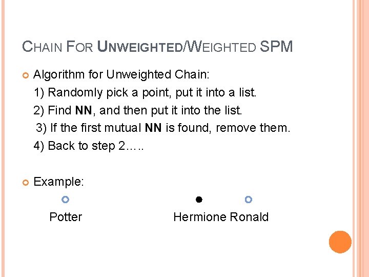
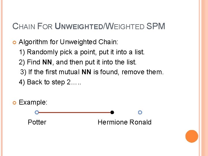
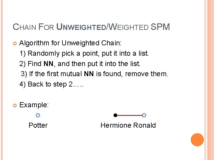
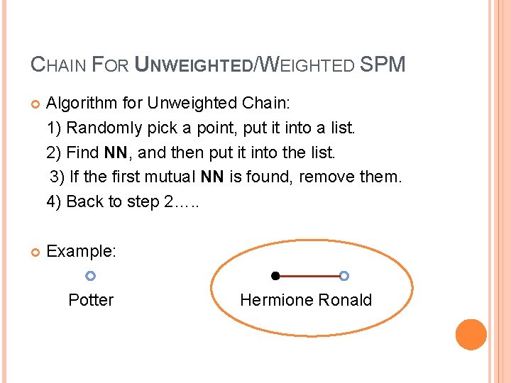
CHAIN FOR UNWEIGHTED/WEIGHTED SPM Algorithm for Unweighted Chain: 1) Randomly pick a point, put it into a list. 2) Find NN, and then put it into the list. 3) If the first mutual NN is found, remove them. 4) Back to step 2…. . Example: Potter Hermione Ronald

CHAIN FOR UNWEIGHTED/WEIGHTED SPM Algorithm for Unweighted Chain: 1) Randomly pick a point, put it into a list. 2) Find NN, and then put it into the list. 3) If the first mutual NN is found, remove them. 4) Back to step 2…. . Example: Potter Hermione Ronald

CHAIN FOR UNWEIGHTED/WEIGHTED SPM Algorithm for Unweighted Chain: 1) Randomly pick a point, put it into a list. 2) Find NN, and then put it into the list. 3) If the first mutual NN is found, remove them. 4) Back to step 2…. . Example: Potter Hermione Ronald

CHAIN FOR UNWEIGHTED/WEIGHTED SPM Algorithm for Unweighted Chain: 1) Randomly pick a point, put it into a list. 2) Find NN, and then put it into the list. 3) If the first mutual NN is found, remove them. 4) Back to step 2…. . Example: Potter Hermione Ronald

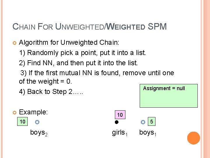
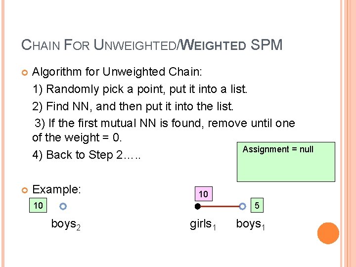
CHAIN FOR UNWEIGHTED/WEIGHTED SPM Algorithm for Unweighted Chain: 1) Randomly pick a point, put it into a list. 2) Find NN, and then put it into the list. 3) If the first mutual NN is found, remove until one of the weight = 0. Assignment = null 4) Back to Step 2…. . Example: 10 10 5 boys 2 girls 1 boys 1

CHAIN FOR UNWEIGHTED/WEIGHTED SPM Algorithm for Unweighted Chain: 1) Randomly pick a point, put it into a list. 2) Find NN, and then put it into the list. 3) If the first mutual NN is found, remove until one of the weight = 0. Assignment = null 4) Back to Step 2…. . Example: 10 10 5 boys 2 girls 1 boys 1

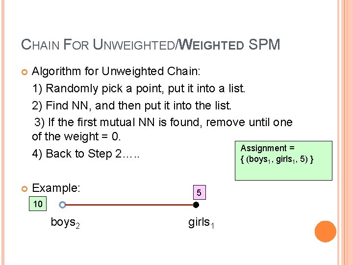
CHAIN FOR UNWEIGHTED/WEIGHTED SPM Algorithm for Unweighted Chain: 1) Randomly pick a point, put it into a list. 2) Find NN, and then put it into the list. 3) If the first mutual NN is found, remove until one of the weight = 0. Assignment = 4) Back to Step 2…. . { (boys , girls , 5) } 1 Example: 5 10 boys 2 girls 1 1

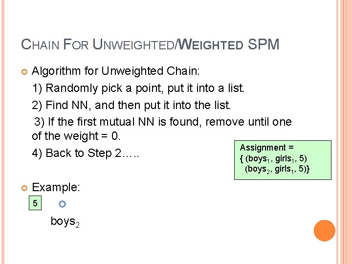
CHAIN FOR UNWEIGHTED/WEIGHTED SPM Algorithm for Unweighted Chain: 1) Randomly pick a point, put it into a list. 2) Find NN, and then put it into the list. 3) If the first mutual NN is found, remove until one of the weight = 0. Assignment = 4) Back to Step 2…. . { (boys , girls , 5) 1 1 (boys 2, girls 1, 5)} Example: 5 boys 2

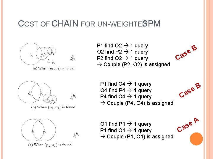
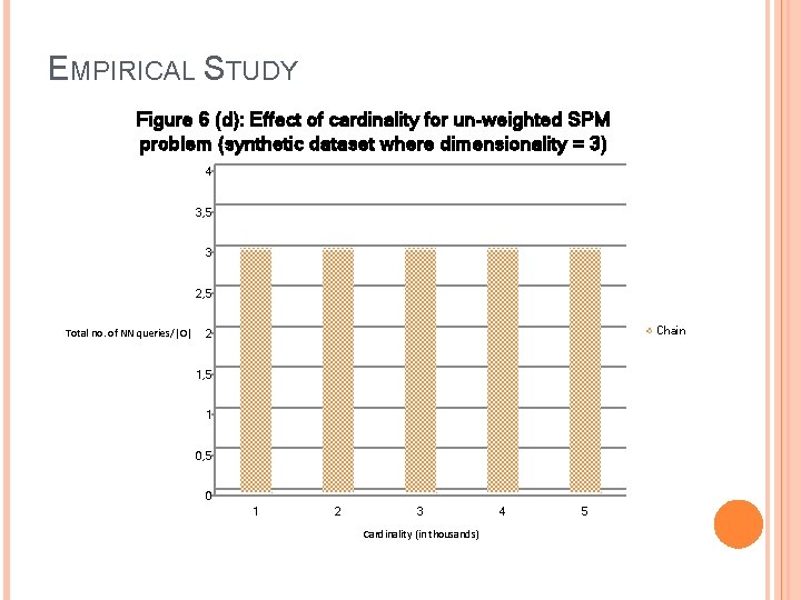
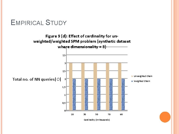
COST OF CHAIN FOR UN-WEIGHTED SPM Theorem 1: Chain performs at most 3|O| NN queries, and exactly 2 |O| object deletions. Proof : At most 3|O| NN queries For each couple (p, o) A, at least 2 queries Each couple (p, o) found by Chain must appear at the end of the chain. Assume that P appears as the last object of the chain O appears as the second last object of the chain

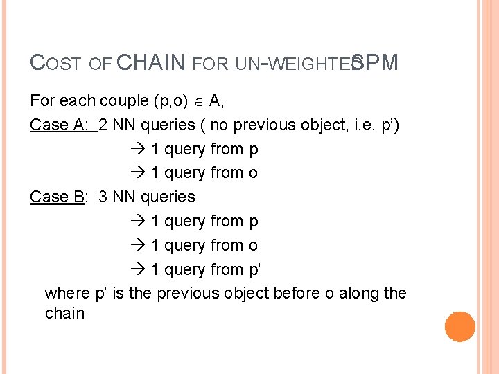
COST OF CHAIN FOR UN-WEIGHTED SPM For each couple (p, o) A, Case A: 2 NN queries ( no previous object, i. e. p’) 1 query from p 1 query from o Case B: 3 NN queries 1 query from p 1 query from o 1 query from p’ where p’ is the previous object before o along the chain

COST OF CHAIN FOR UN-WEIGHTED SPM P 1 find O 2 1 query O 2 find P 2 1 query P 2 find O 2 1 query Couple (P 2, O 2) is assigned P 1 find O 4 1 query O 4 find P 4 1 query P 4 find O 4 1 query Couple (P 4, O 4) is assigned O 1 find P 1 1 query P 1 find O 1 1 query Couple (P 1, O 1) is assigned B e as C C A e as

COST OF CHAIN FOR UN-WEIGHTED SPM Since |P| > |O|, |O| couple in assignment Thus, At most 3|O| NN queries Proof: exactly 2 |O| object deletions When find a couple, delete 1 object from P delete 1 object from O Since |O| couple in assignment Thus, exactly 2 |O| object deletions

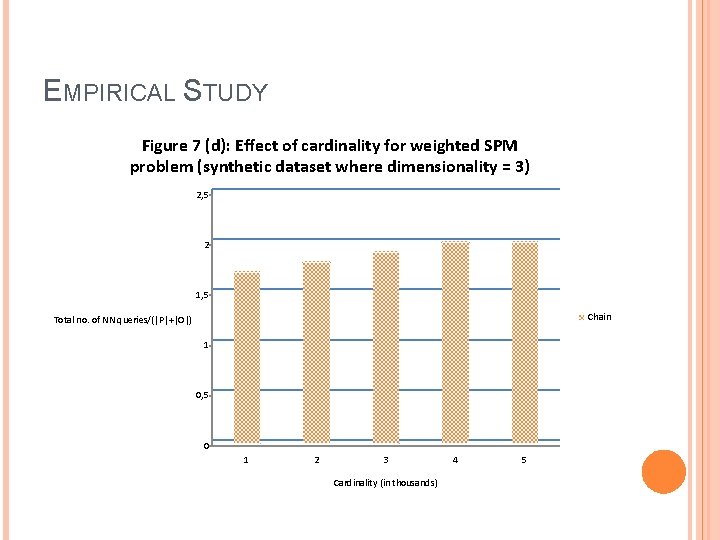
COST OF CHAIN FOR WEIGHTED SPM Theorem 3: Weighted Chain performs at most 3(|P| + |O|) NN queries, and at most |P| + |O| object deletions. Proof: At most 3(|P| + |O|) NN queries - 3 NN queries for each extended couple (p, o, w) - Remove only one object from its origin dataset total No. of couples (p, o, w) <= |P| + |O| Thus, at most 3(|P| + |O|) NN queries Proof: At most |P| + |O| deletions - Remove only one object from its origin dataset Thus, total deletions <= |P| + |O|

RUNNING TIME OF CHAIN (|N|) = complexity of NN query (|N|) = object deletion For Un-weighted SPM Running time of Chain = O(|O|. ( (|P|)+ (|P|))) If randomized technique (one of NN queries) used, (|P|) = log 2 (|P|) = log (|P|) Thus, in this case, time complexity of Chain = O(|O|. log. O(1)|P|)

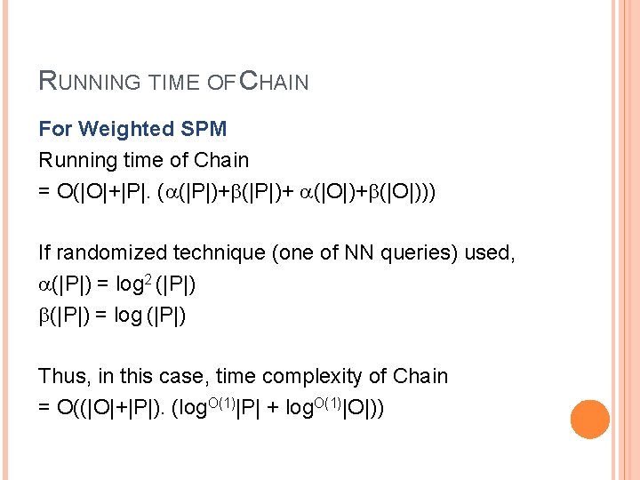
RUNNING TIME OF CHAIN For Weighted SPM Running time of Chain = O(|O|+|P|. ( (|P|)+ (|O|)+ (|O|))) If randomized technique (one of NN queries) used, (|P|) = log 2 (|P|) = log (|P|) Thus, in this case, time complexity of Chain = O((|O|+|P|). (log. O(1)|P| + log. O(1)|O|))

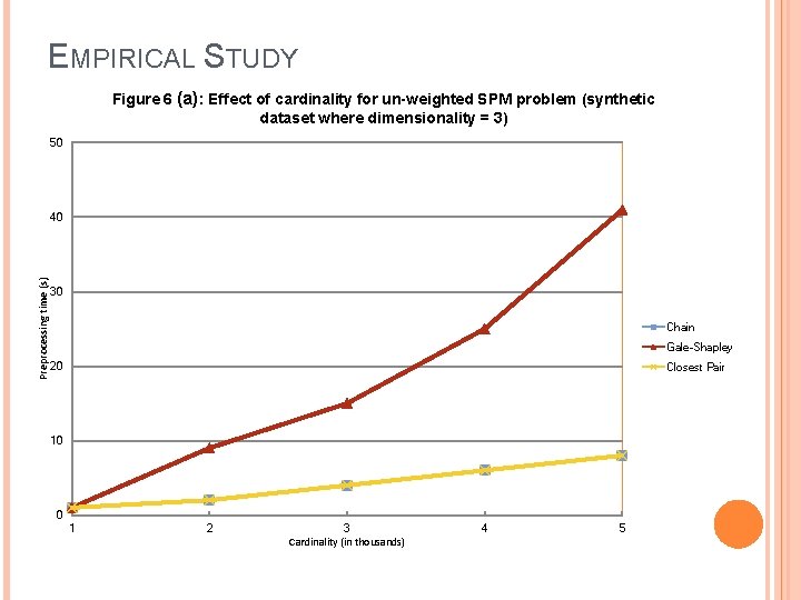
EMPIRICAL STUDY Figure 6 (a): Effect of cardinality for un-weighted SPM problem (synthetic dataset where dimensionality = 3) 50 Preprocessing time (s) 40 30 Chain Gale-Shapley 20 Closest Pair 10 0 1 2 3 Cardinality (in thousands) 4 5

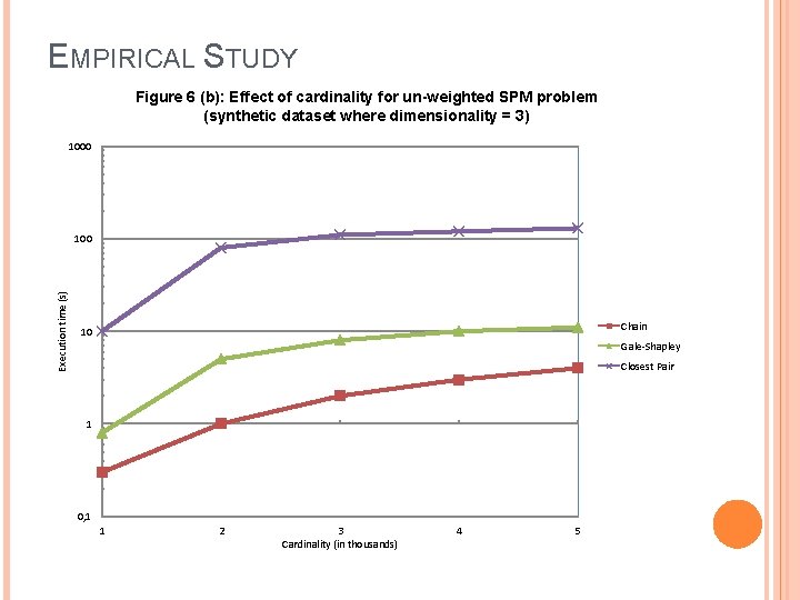
EMPIRICAL STUDY Figure 6 (b): Effect of cardinality for un-weighted SPM problem (synthetic dataset where dimensionality = 3) 1000 Execution time (s) 100 Chain 10 Gale-Shapley Closest Pair 1 0, 1 1 2 3 Cardinality (in thousands) 4 5

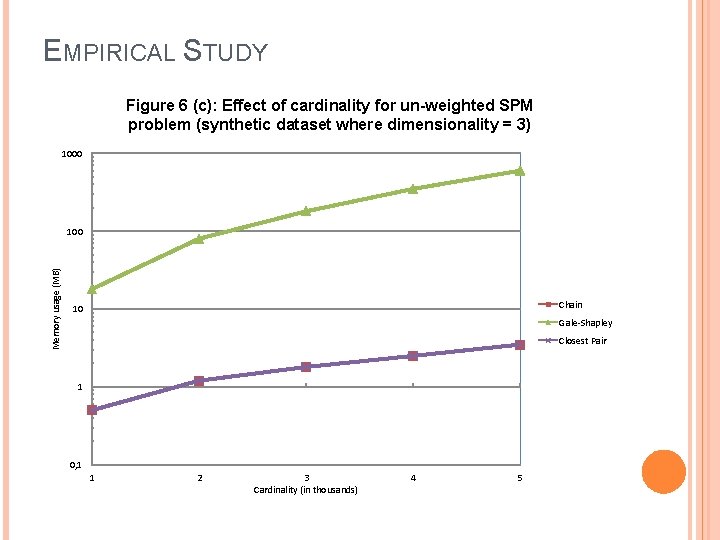
EMPIRICAL STUDY Figure 6 (c): Effect of cardinality for un-weighted SPM problem (synthetic dataset where dimensionality = 3) 1000 Memory usage (MB) 100 Chain 10 Gale-Shapley Closest Pair 1 0, 1 1 2 3 Cardinality (in thousands) 4 5

EMPIRICAL STUDY Figure 6 (d): Effect of cardinality for un-weighted SPM problem (synthetic dataset where dimensionality = 3) 4 3, 5 3 2, 5 Total no. of NN queries/|O| Chain 2 1, 5 1 0, 5 0 1 2 3 Cardinality (in thousands) 4 5

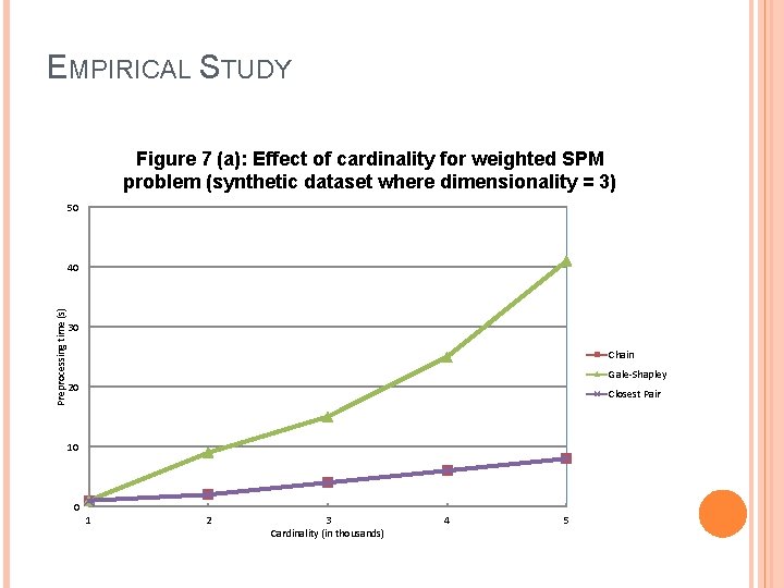
EMPIRICAL STUDY Figure 7 (a): Effect of cardinality for weighted SPM problem (synthetic dataset where dimensionality = 3) 50 Preprocessing time (s) 40 30 Chain Gale-Shapley 20 Closest Pair 10 0 1 2 3 Cardinality (in thousands) 4 5

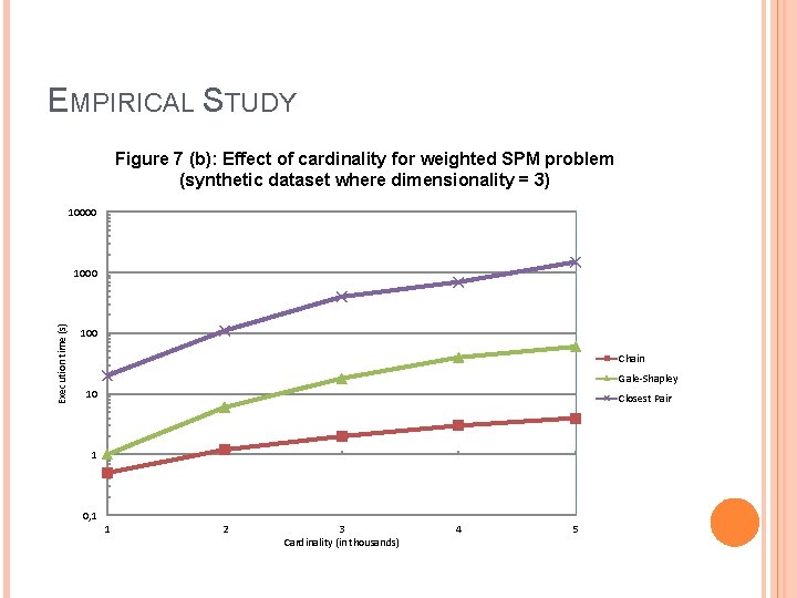
EMPIRICAL STUDY Figure 7 (b): Effect of cardinality for weighted SPM problem (synthetic dataset where dimensionality = 3) 10000 Execution time (s) 1000 100 Chain Gale-Shapley 10 Closest Pair 1 0, 1 1 2 3 Cardinality (in thousands) 4 5

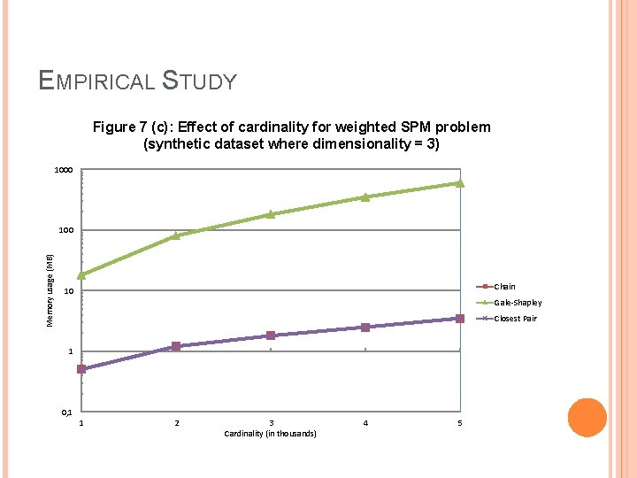
EMPIRICAL STUDY Figure 7 (c): Effect of cardinality for weighted SPM problem (synthetic dataset where dimensionality = 3) 1000 Memory usage (MB) 100 Chain 10 Gale-Shapley Closest Pair 1 0, 1 1 2 3 Cardinality (in thousands) 4 5

EMPIRICAL STUDY Figure 7 (d): Effect of cardinality for weighted SPM problem (synthetic dataset where dimensionality = 3) 2, 5 2 1, 5 Chain Total no. of NN queries/(|P|+|O|) 1 0, 5 0 1 2 3 Cardinality (in thousands) 4 5

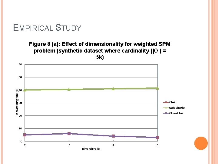
EMPIRICAL STUDY Figure 8 (a): Effect of dimensionality for weighted SPM problem (synthetic dataset where cardinality (|O|) = 5 k) 60 Preprocessing time (s) 50 40 Chain 30 Gale-Shapley Closest Pair 20 10 0 2 3 Dimensionality 4 5

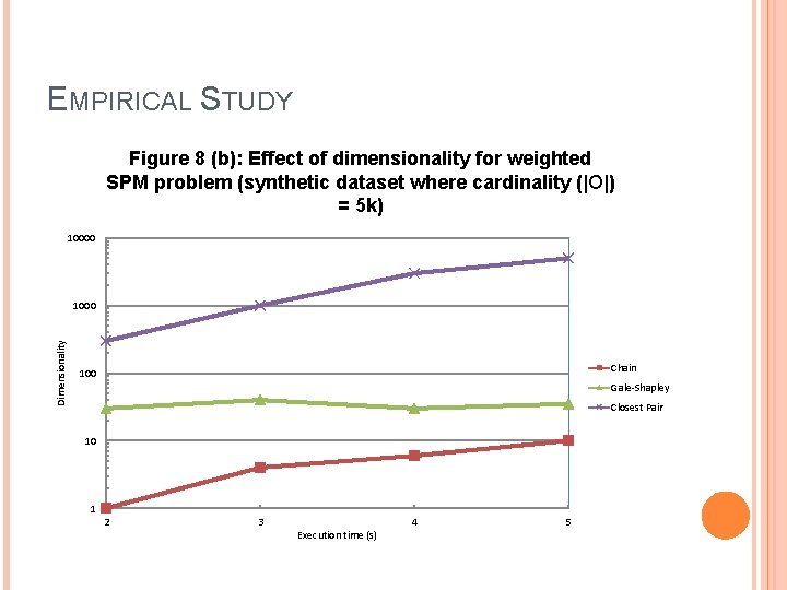
EMPIRICAL STUDY Figure 8 (b): Effect of dimensionality for weighted SPM problem (synthetic dataset where cardinality (|O|) = 5 k) 10000 Dimensionality 1000 Chain 100 Gale-Shapley Closest Pair 10 1 2 3 Execution time (s) 4 5

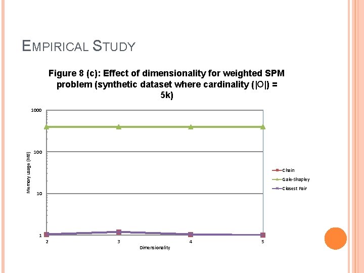
EMPIRICAL STUDY Figure 8 (c): Effect of dimensionality for weighted SPM problem (synthetic dataset where cardinality (|O|) = 5 k) Memory usage (MB) 1000 100 Chain Gale-Shapley Closest Pair 10 1 2 3 Dimensionality 4 5

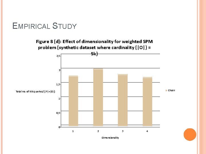
EMPIRICAL STUDY Figure 8 (d): Effect of dimensionality for weighted SPM problem (synthetic dataset where cardinality (|O|) = 5 k) 2, 5 2 1, 5 Chain Total no. of NN queries/(|P|+|O|) 1 0, 5 0 1 2 3 Dimensionality 4

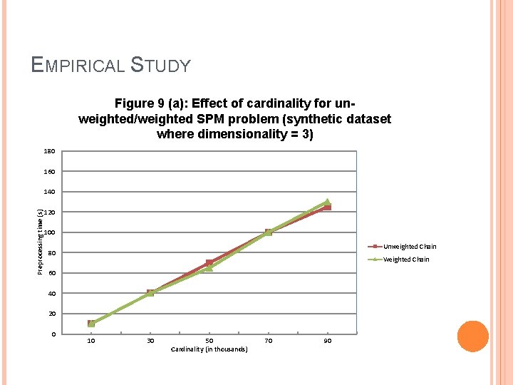
EMPIRICAL STUDY Figure 9 (a): Effect of cardinality for unweighted/weighted SPM problem (synthetic dataset where dimensionality = 3) 180 160 Preprocessing time (s) 140 120 100 Unweighted Chain 80 Weighted Chain 60 40 20 0 10 30 50 Cardinality (in thousands) 70 90

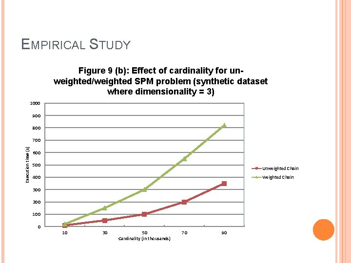
EMPIRICAL STUDY Figure 9 (b): Effect of cardinality for unweighted/weighted SPM problem (synthetic dataset where dimensionality = 3) 1000 900 800 Execution time (s) 700 600 500 Unweighted Chain Weighted Chain 400 300 200 100 0 10 30 50 Cardinality (in thousands) 70 90

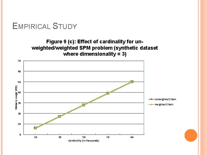
EMPIRICAL STUDY Figure 9 (c): Effect of cardinality for unweighted/weighted SPM problem (synthetic dataset where dimensionality = 3) 70 60 Memory usage (MB) 50 40 Unweighted Chain 30 Weighted Chain 20 10 30 50 Cardinality (in thousands) 70 90

EMPIRICAL STUDY Figure 9 (d): Effect of cardinality for unweighted/weighted SPM problem (synthetic dataset where dimensionality = 3) 4 3, 5 3 2, 5 Total no. of NN queries|O| Unweighted Chain 2 Weighted Chain 1, 5 1 0, 5 0 10 30 50 70 Cardinality (in thousands) 90

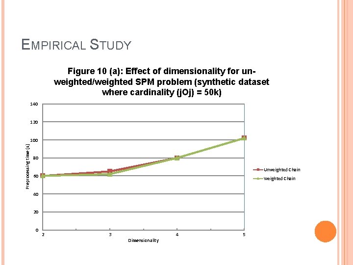
EMPIRICAL STUDY Figure 10 (a): Effect of dimensionality for unweighted/weighted SPM problem (synthetic dataset where cardinality (j. Oj) = 50 k) 140 120 Preprocessing time (s) 100 80 Unweighted Chain 60 Weighted Chain 40 20 0 2 3 Dimensionality 4 5

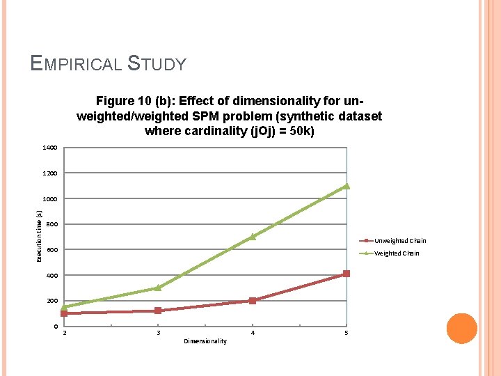
EMPIRICAL STUDY Figure 10 (b): Effect of dimensionality for unweighted/weighted SPM problem (synthetic dataset where cardinality (j. Oj) = 50 k) 1400 1200 Execution time (s) 1000 800 Unweighted Chain 600 Weighted Chain 400 200 0 2 3 Dimensionality 4 5

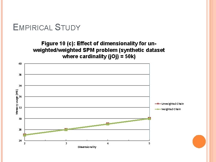
EMPIRICAL STUDY Figure 10 (c): Effect of dimensionality for unweighted/weighted SPM problem (synthetic dataset where cardinality (j. Oj) = 50 k) 40 38 Memory usage (MB) 36 34 Unweighted Chain 32 Weighted Chain 30 28 26 2 3 Dimensionality 4 5

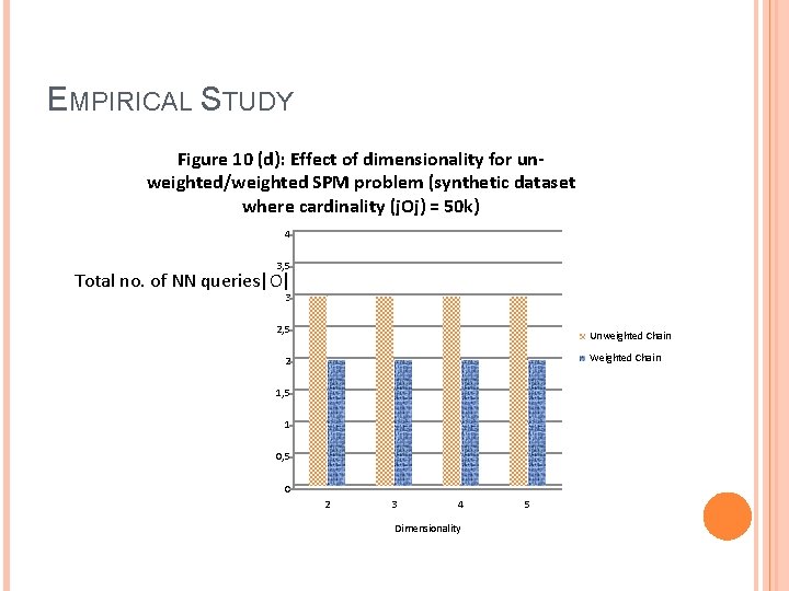
EMPIRICAL STUDY Figure 10 (d): Effect of dimensionality for unweighted/weighted SPM problem (synthetic dataset where cardinality (j. Oj) = 50 k) 4 3, 5 Total no. of NN queries|O| 3 2, 5 Unweighted Chain Weighted Chain 2 1, 5 1 0, 5 0 2 3 4 Dimensionality 5

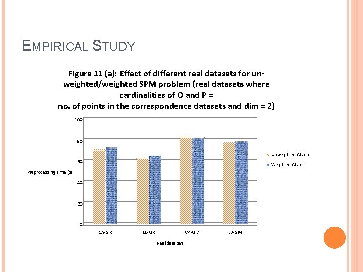
EMPIRICAL STUDY Figure 11 (a): Effect of different real datasets for unweighted/weighted SPM problem (real datasets where cardinalities of O and P = no. of points in the correspondence datasets and dim = 2) 100 80 Unweighted Chain 60 Weighted Chain Preprocessing time (s) 40 20 0 CA-GR LB-GR CA-GM Real data set LB-GM

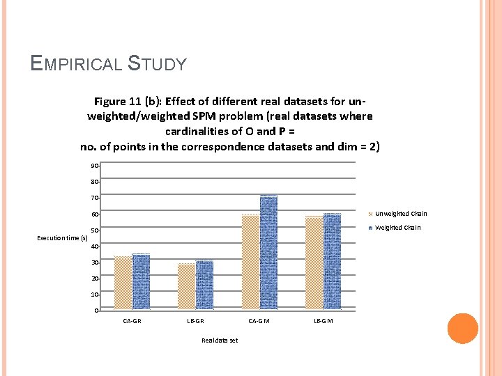
EMPIRICAL STUDY Figure 11 (b): Effect of different real datasets for unweighted/weighted SPM problem (real datasets where cardinalities of O and P = no. of points in the correspondence datasets and dim = 2) 90 80 70 Execution time (s) 60 Unweighted Chain 50 Weighted Chain 40 30 20 10 0 CA-GR LB-GR Real data set CA-GM LB-GM

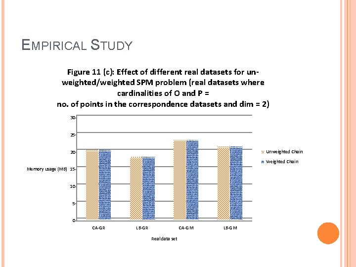
EMPIRICAL STUDY Figure 11 (c): Effect of different real datasets for unweighted/weighted SPM problem (real datasets where cardinalities of O and P = no. of points in the correspondence datasets and dim = 2) 30 25 Unweighted Chain 20 Weighted Chain Memory usage (MB) 15 10 5 0 CA-GR LB-GR CA-GM Real data set LB-GM

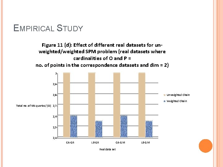
EMPIRICAL STUDY Figure 11 (d): Effect of different real datasets for unweighted/weighted SPM problem (real datasets where cardinalities of O and P = no. of points in the correspondence datasets and dim = 2) 3 2, 9 Unweighted Chain 2, 8 Weighted Chain Total no. of NN queries/|O| 2, 7 2, 6 2, 5 2, 4 CA-GR LB-GR CA-GM Real data set LB-GM

CONCLUSION Un-weighted and Weighted Spatial Matching Problem �A generalization of BRNN � Un-weighted SPM can be extended to Weighted SPM Algorithm Chain � Improvement on Running Time