OMGT 1117 LECTURE 11 Simple Correlation and Regression

OMGT 1117 - LECTURE 11: Simple Correlation and Regression Analysis Reading Property Data Analysis – A Primer, Ch. 11

Objectives • Describe the Simple Linear Population Regression Model and the Classical Assumptions. • Explain how one interprets and obtains the Sample Regression Line using the least squares estimation procedure. • Consider point prediction issues in respect of interpolation and extrapolation • Summarise the attributes of the Least Squares estimators when the classical assumptions hold and briefly consider the implications if the assumptions are violated • Distinguish between cross-sectional and time series data • Explain how to calculate and interpret the standard error of estimate and the coefficient of determination. • Explain how to calculate and interpret the Coefficient of Correlation • Highlight various caveats regarding Regression and Correlation Analysis Slide 2

Introduction In today’s lecture two related techniques are considered: Simple Linear Regression Where the linear relationship between Y (say price of apartment) and X (say apartment gross rental) is estimated Simple Correlation Analysis Where the strength of linear association between two variables X and Y is measured Slide 3

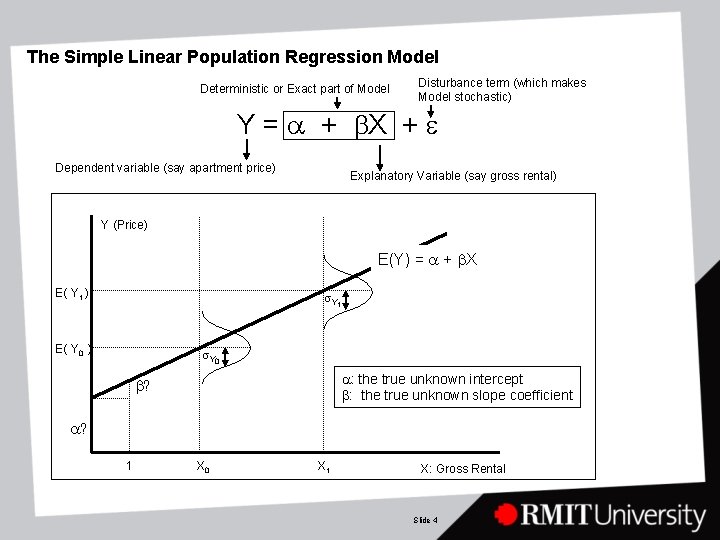
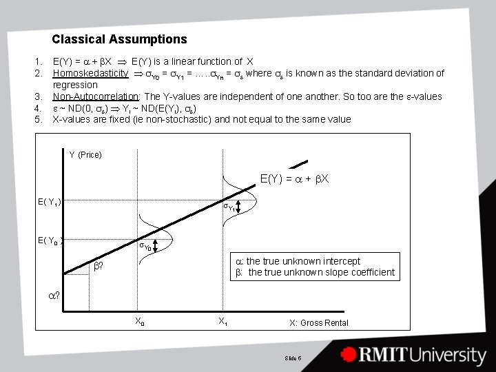
The Simple Linear Population Regression Model Deterministic or Exact part of Model Disturbance term (which makes Model stochastic) Y = a + b. X + e Dependent variable (say apartment price) Explanatory Variable (say gross rental) Y (Price) E(Y) = a + b. X E( Y 1 ) s. Y 1 E( Y 0 ) s. Y 0 a: the true unknown intercept b: the true unknown slope coefficient b? a? 1 X 0 X 1 X: Gross Rental Slide 4

Classical Assumptions 1. 2. 3. 4. 5. E(Y) = a + b. X E(Y) is a linear function of X Homoskedasticity s. Y 0 = s. Y 1 = …. . s. Yn = se where se is known as the standard deviation of regression Non-Autocorrelation: The Y-values are independent of one another. So too are the e-values e ~ ND(0, se) Yi ~ ND(E(Yi), se) X-values are fixed (ie non-stochastic) and not equal to the same value Y (Price) E(Y) = a + b. X E( Y 1 ) s. Y 1 E( Y 0 ) s. Y 0 a: the true unknown intercept b: the true unknown slope coefficient b? a? X 0 X 1 X: Gross Rental Slide 5

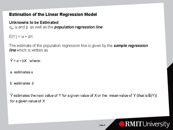
Estimation of the Linear Regression Model Unknowns to be Estimated: se, a and b as well as the population regression line: E(Y) = a + b. X The estimate of the population regression line is given by the sample regression line which is written as Slide 6

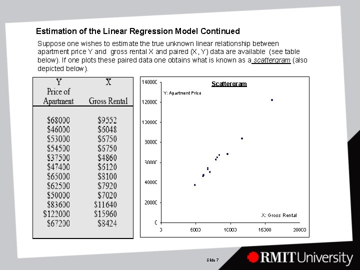
Estimation of the Linear Regression Model Continued Suppose one wishes to estimate the true unknown linear relationship between apartment price Y and gross rental X and paired (X, Y) data are available (see table below). If one plots these paired data one obtains what is known as a scattergram (also depicted below). Scattergram Y: Apartment Price X: Gross Rental Slide 7

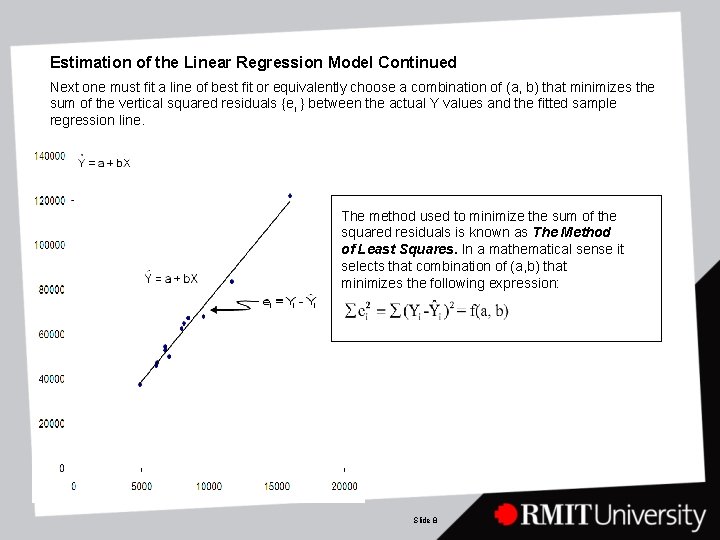
Estimation of the Linear Regression Model Continued Next one must fit a line of best fit or equivalently choose a combination of (a, b) that minimizes the sum of the vertical squared residuals {ei } between the actual Y values and the fitted sample regression line. The method used to minimize the sum of the squared residuals is known as The Method of Least Squares. In a mathematical sense it selects that combination of (a, b) that minimizes the following expression: Slide 8

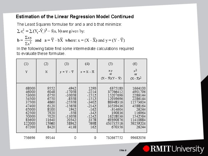
Estimation of the Linear Regression Model Continued The Least Squares formulae for and a and b that minimize: In the following table find some intermediate calculations required to evaluate these formulae. Slide 9

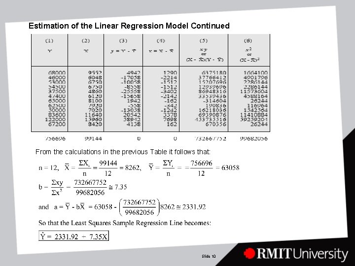
Estimation of the Linear Regression Model Continued From the calculations in the previous Table it follows that: Slide 10

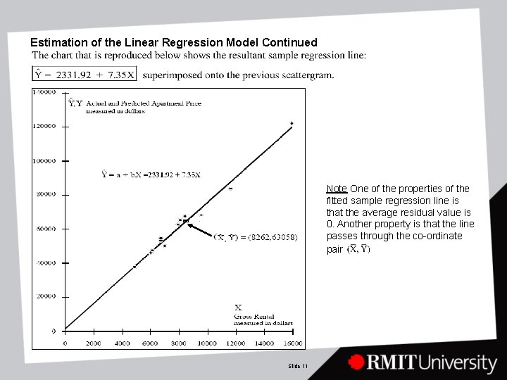
Estimation of the Linear Regression Model Continued Note One of the properties of the fitted sample regression line is that the average residual value is 0. Another property is that the line passes through the co-ordinate pair Slide 11

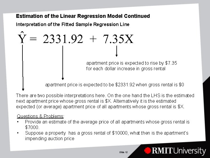
Estimation of the Linear Regression Model Continued Interpretation of the Fitted Sample Regression Line apartment price is expected to rise by $7. 35 for each dollar increase in gross rental apartment price is expected to be $2331. 92 when gross rental is $0 There are two possible interpretations here. On the one hand the LHS is the estimated next apartment price whose gross rental is $X. Alternatively it is the estimated expected (or average) apartment price of all apartments whose gross rental is $X. Questions & Problems: • Provide an estimate of the average price of all apartments whose gross rental is $7000. • Suppose a property has a gross rental of $10000, what then is the apartment’s impending auction price Slide 12

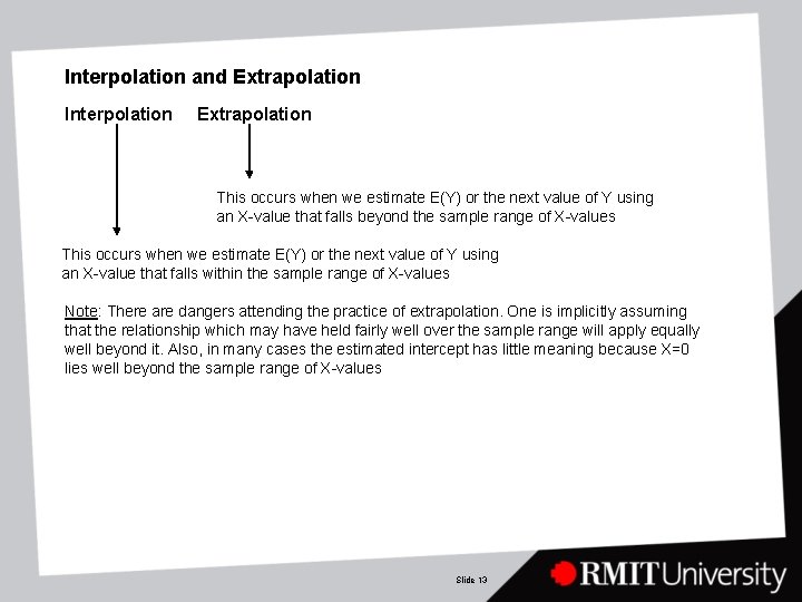
Interpolation and Extrapolation Interpolation Extrapolation This occurs when we estimate E(Y) or the next value of Y using an X-value that falls beyond the sample range of X-values This occurs when we estimate E(Y) or the next value of Y using an X-value that falls within the sample range of X-values Note: There are dangers attending the practice of extrapolation. One is implicitly assuming that the relationship which may have held fairly well over the sample range will apply equally well beyond it. Also, in many cases the estimated intercept has little meaning because X=0 lies well beyond the sample range of X-values Slide 13

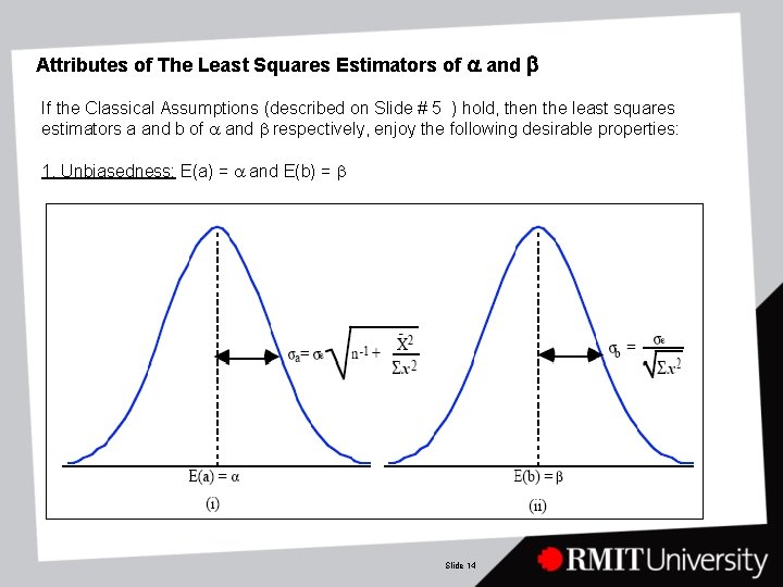
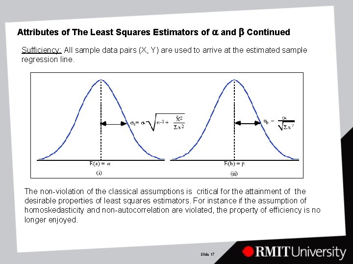
Attributes of The Least Squares Estimators of a and b If the Classical Assumptions (described on Slide # 5 ) hold, then the least squares estimators a and b of a and b respectively, enjoy the following desirable properties: 1. Unbiasedness: E(a) = a and E(b) = b Slide 14

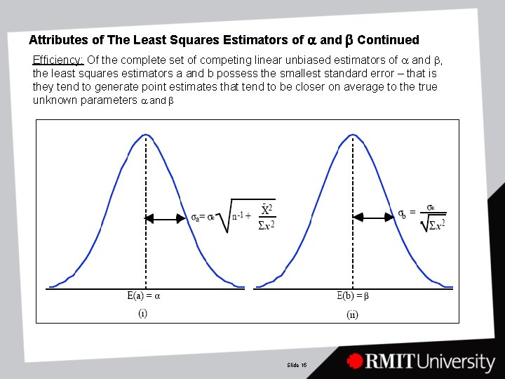
Attributes of The Least Squares Estimators of a and b Continued Efficiency: Of the complete set of competing linear unbiased estimators of a and b, the least squares estimators a and b possess the smallest standard error – that is they tend to generate point estimates that tend to be closer on average to the true unknown parameters a and b Slide 15

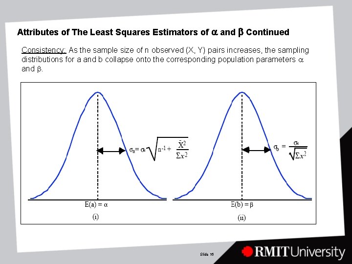
Attributes of The Least Squares Estimators of a and b Continued Consistency: As the sample size of n observed (X, Y) pairs increases, the sampling distributions for a and b collapse onto the corresponding population parameters a and b. Slide 16

Attributes of The Least Squares Estimators of a and b Continued Sufficiency: All sample data pairs (X, Y) are used to arrive at the estimated sample regression line. The non-violation of the classical assumptions is critical for the attainment of the desirable properties of least squares estimators. For instance if the assumption of homoskedasticity and non-autocorrelation are violated, the property of efficiency is no longer enjoyed. Slide 17

Data Most Susceptible to Heteroskedasticity and Auto-Correlation Time Series Data: These are data gathered over time. These data are often associated with auto-correlation sometimes referred to as serial correlation. Cross-Sectional Data: The data are gathered across individuals, objects or space at a specific point in time. These data are often associated with the violation of homoskedasticity (often referred to as heteroskedasticity) Pooled or Panel Data: These data are simultaneously cross-sectional and temporal and may be affected by both serial correlation and heteroskedasticity. When the classical assumptions are violated one has to either transform the data (ie correct the data) before they may be meaningfully used for a least squares estimation process. Alternatively, a totally different estimation methodology may be invoked. The former remedy is touched upon in the next topic. The second course of action is well beyond the scope of the present course. Slide 18

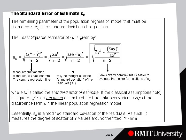
The Standard Error of Estimate se The remaining parameter of the population regression model that must be estimated is se : the standard deviation of regression. The Least Squares estimator of se is given by: Measures the variation of the actual Y-values from The sample regression line May be thought of as the “standard deviation” of the residuals { ei } Looks overly complex but is easier to evaluate than other formulations of se where se is called the standard error of estimate. If the classical assumptions hold, its square se 2 is an unbiased estimate of the true unknown variance se 2 of the disturbance-term e in the linear population regression model. Essentially, se is a modified standard deviation of the residuals. As such, it measures the degree of scatter of Y-values around the fitted Slide 19

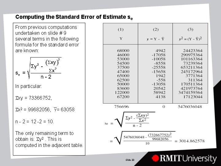
Computing the Standard Error of Estimate se From previous computations undertaken on slide # 9 several terms in the following formula for the standard error are known: In particular: Sxy = 73366752, Sx 2 = 99682056, Y= 63058 n - 2 = 12 -2 = 10. The only remaining term to obtain is: Sy 2. This is computed in the adjacent table. Slide 20

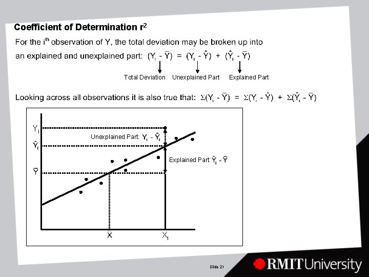
Coefficient of Determination r 2 Total Deviation Yi Unexplained Part: Explained Part: Xi Slide 21 Explained Part

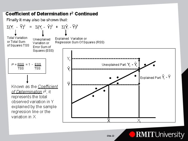
Coefficient of Determination r 2 Continued Total Variation or Total Sum of Squares TSS Explained Variation or Unexplained Regression Sum Of Squares (RSS) Variation or Error Sum of Squares (ESS) Yi r 2 = RSS = 1 - ESS TSS Unexplained Part: Explained Part: Known as the Coefficient of Determination r 2, it represents the total observed variation in Y explained by the sample regression line or the variation in X Xi Slide 22

Calculating the Coefficient of Determination r 2 So 98% of the variation in apartment prices may be explained by the fitted regression line or variation in gross rental figures. NB 0 r 2 1 The closer is r 2 to unity (zero), the better (worse) is the fit of the sample regression line to the points in the scattergram Slide 23

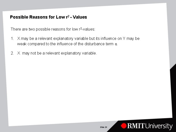
Possible Reasons for Low r 2 - Values There are two possible reasons for low r 2 -values: 1. X may be a relevant explanatory variable but its influence on Y may be weak compared to the influence of the disturbance term e. 2. X may not be a relevant explanatory variable. Slide 24

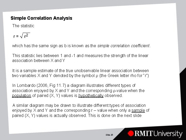
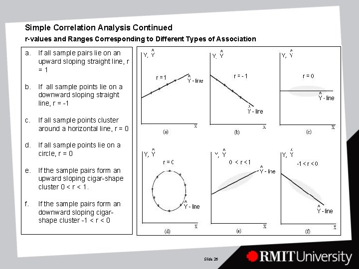
Simple Correlation Analysis The statistic which has the same sign as b is known as the simple correlation coefficient. This statistic lies between 1 and -1 and measures the strength of the linear association between X and Y It is a sample estimate of the true unobservable linear association between two variables X and Y denoted by the symbol r (the Greek letter rho for “r”) In Lombardo (2006, Fig 11. 7) a diagram illustrates different types of association enjoyed by X and Y and the corresponding r-value when the population of paired (X, Y) values is hypothetically observed. A similar diagram may be drawn to illustrate different types of association enjoyed by X and Y and the corresponding r – value when only a sample of paired (X, Y) values is actually observed. This is done on the next slide Slide 25

Simple Correlation Analysis Continued r-values and Ranges Corresponding to Different Types of Association a. If all sample pairs lie on an upward sloping straight line, r =1 b. If all sample points lie on a downward sloping straight line, r = -1 c. If all sample points cluster around a horizontal line, r = 0 d. If all sample points lie on a circle, r = 0 e. If the sample pairs form an upward sloping cigar-shape cluster 0 < r < 1. f. If the sample pairs form an downward sloping cigarshape cluster -1 < r < 0 Slide 26

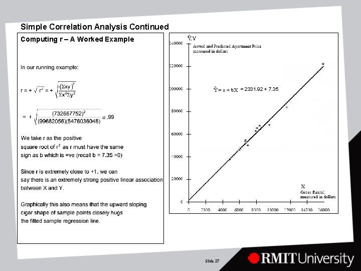
Simple Correlation Analysis Continued Computing r – A Worked Example = 2331. 92 + 7. 35 Slide 27

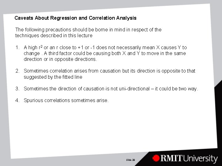
Caveats About Regression and Correlation Analysis The following precautions should be borne in mind in respect of the techniques described in this lecture 1. A high r 2 or an r close to +1 or -1 does not necessarily mean X causes Y to change. A third factor could be causing both X and Y to move in the same direction or in opposite directions. 2. Sometimes correlation arises from causation but its direction is opposite to that suggested by the fitted line 3. Sometimes the direction of causation is not uni-directional – it could be two way. 4. Spurious correlations sometimes arise. Slide 28

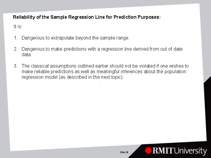
Reliability of the Sample Regression Line for Prediction Purposes: It is: 1. Dangerous to extrapolate beyond the sample range. 2. Dangerous to make predictions with a regression line derived from out of date data 3. The classical assumptions outlined earlier should not be violated if one wishes to make reliable predictions as well as meaningful inferences about the population regression model (as described in the next topic). Slide 29

The Choice between Conducting Regression or Correlation Analysis: Regression may be regarded as the preferred technique because: 1. It provides more information on the nature of the relationship between X and Y 2. The assumptions that validate correlation are far more restrictive than those validating Regression Analysis. Slide 30