OLN Introduction to Linear Programming 12312021 1 Overview

OLN Introduction to Linear Programming 12/31/2021 1

Overview Linear Programming (LP): – Is a standard tool in industry, commerce, and government – Has led to millions of dollars of savings for many organizations. – Is concerned with allocating limited resources among competing activities in an optimal way. – Employs a math model in which all functions are linear – The term programming implies planning – Uses very efficient solution procedures such as the simplex method. – Has been successfully applied to an incredibly wide variety of problems – Is a conceptual foundation for other types of optimization procedures. 12/31/2021 rd 2

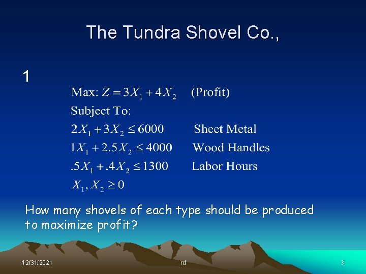
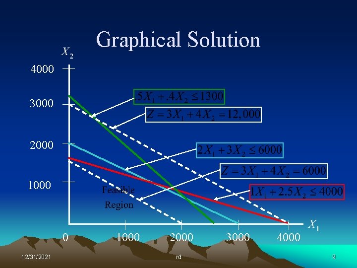
The Tundra Shovel Co. , 1 How many shovels of each type should be produced to maximize profit? 12/31/2021 rd 3

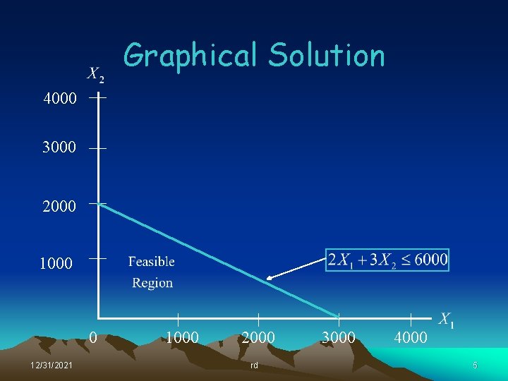
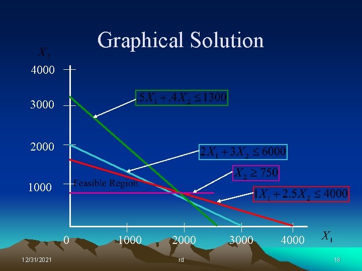
Graphical Solution 4000 3000 2000 1000 0 12/31/2021 1000 2000 rd 3000 4

Graphical Solution 4000 3000 2000 1000 0 12/31/2021 1000 2000 rd 3000 4000 5

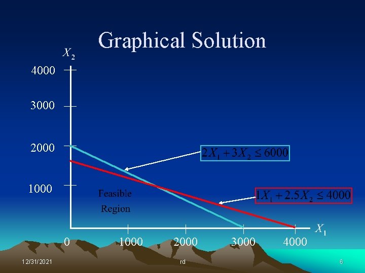
Graphical Solution 4000 3000 2000 1000 0 12/31/2021 1000 2000 rd 3000 4000 6

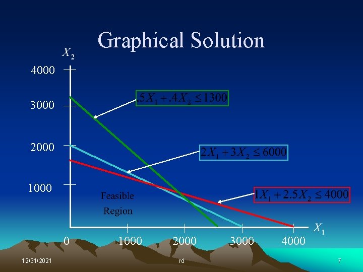
Graphical Solution 4000 3000 2000 1000 0 12/31/2021 1000 2000 rd 3000 4000 7

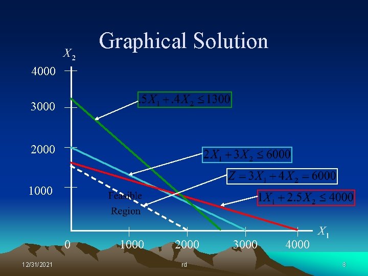
Graphical Solution 4000 3000 2000 1000 0 12/31/2021 1000 2000 rd 3000 4000 8

Graphical Solution 4000 3000 2000 1000 0 12/31/2021 1000 2000 rd 3000 4000 9

Graphical Solution 4000 3000 2000 1000 0 12/31/2021 1000 2000 rd 3000 4000 10

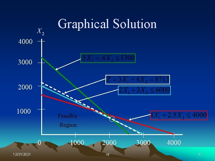
Graphical Solution 4000 3000 2000 1000 0 12/31/2021 1000 2000 rd 3000 4000 11

Lessons Learned So what did we learn form this graphical exercise? • The optimal solution always lies at a corner point of the feasible region. • A corner point is defined by the intersection of at least two constraints – The resources represented by these corner-point constraints will be totally consumed by the optimal solution. – Resources represented by constraint lines that do not pass through the optimal point will not be totally consumed. • We really don’t want to graph large problems! 12/31/2021 rd 12

A Slight Diversion The preceding slides showed a graphical solution procedure for LP’s. – Only works with two decision variables – It is primarily conceptual, to help you understand what is going on behind the scenes – The OR Tutor software accompanying the text illustrates the graphical method on other examples We will primarily use the Simplex method for solving problems – Implemented in the Excel Solver, LINGO/LINDO, and MPL/CPLEX, as described in the text – All meaningful applications are solved using a software package 12/31/2021 rd 13

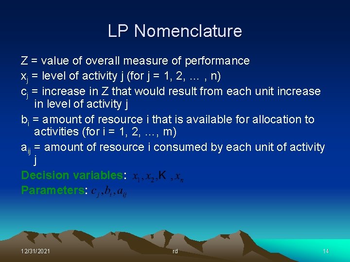
LP Nomenclature Z = value of overall measure of performance xj = level of activity j (for j = 1, 2, … , n) cj = increase in Z that would result from each unit increase in level of activity j bi = amount of resource i that is available for allocation to activities (for i = 1, 2, …, m) aij = amount of resource i consumed by each unit of activity j Decision variables: Parameters: 12/31/2021 rd 14

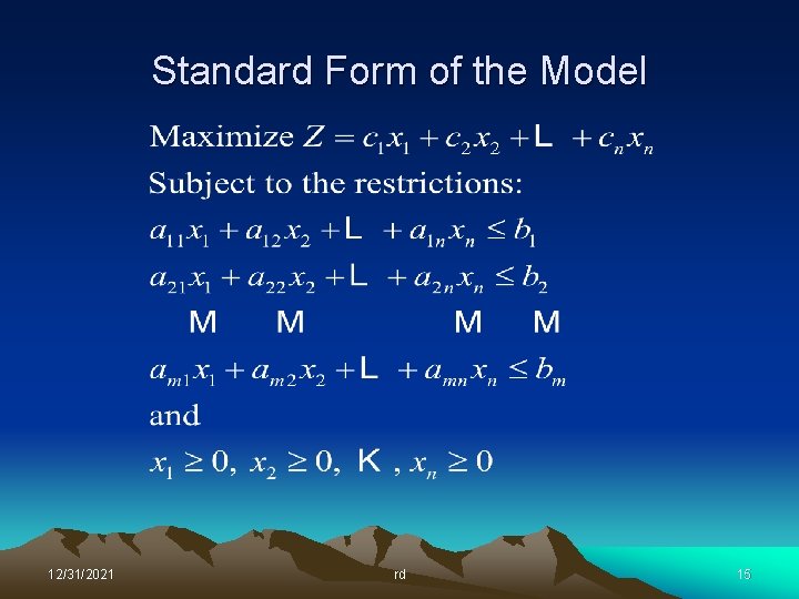
Standard Form of the Model 12/31/2021 rd 15

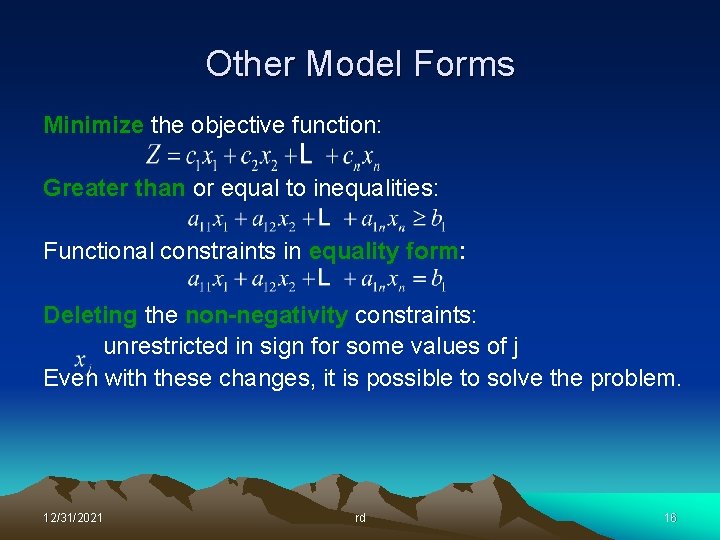
Other Model Forms Minimize the objective function: Greater than or equal to inequalities: Functional constraints in equality form: Deleting the non-negativity constraints: unrestricted in sign for some values of j Even with these changes, it is possible to solve the problem. 12/31/2021 rd 16

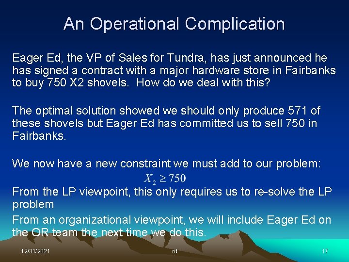
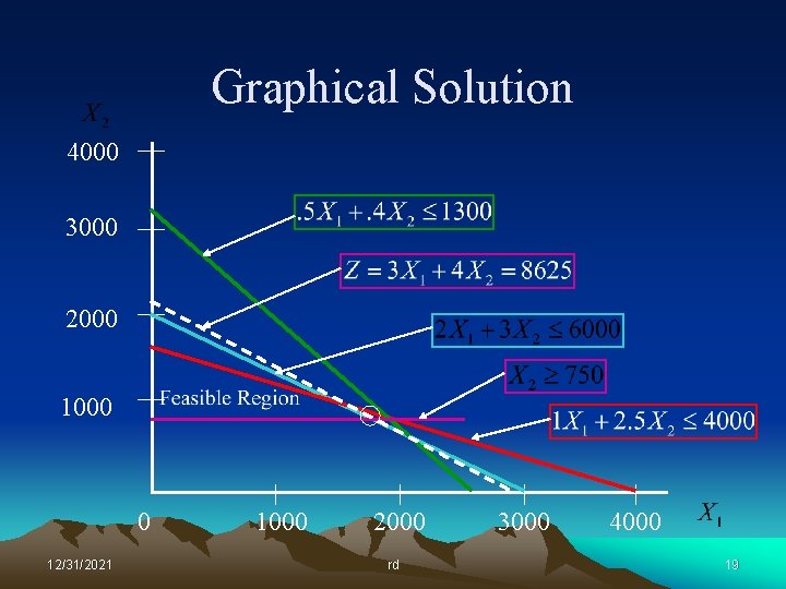
An Operational Complication Eager Ed, the VP of Sales for Tundra, has just announced he has signed a contract with a major hardware store in Fairbanks to buy 750 X 2 shovels. How do we deal with this? The optimal solution showed we should only produce 571 of these shovels but Eager Ed has committed us to sell 750 in Fairbanks. We now have a new constraint we must add to our problem: From the LP viewpoint, this only requires us to re-solve the LP problem From an organizational viewpoint, we will include Eager Ed on the OR team the next time we do this. 12/31/2021 rd 17

Graphical Solution 4000 3000 2000 1000 0 12/31/2021 1000 2000 rd 3000 4000 18

Graphical Solution 4000 3000 2000 1000 0 12/31/2021 1000 2000 rd 3000 4000 19

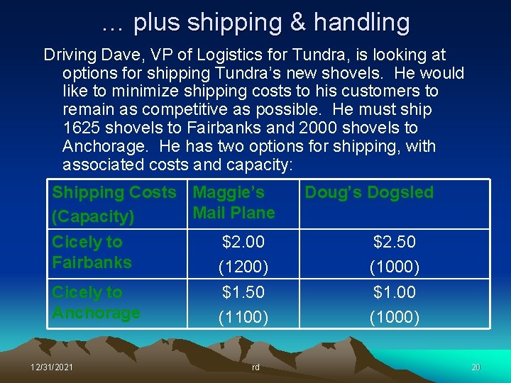
… plus shipping & handling Driving Dave, VP of Logistics for Tundra, is looking at options for shipping Tundra’s new shovels. He would like to minimize shipping costs to his customers to remain as competitive as possible. He must ship 1625 shovels to Fairbanks and 2000 shovels to Anchorage. He has two options for shipping, with associated costs and capacity: Shipping Costs Maggie’s Mail Plane (Capacity) Cicely to $2. 00 Fairbanks (1200) Cicely to Anchorage 12/31/2021 $1. 50 (1100) rd Doug’s Dogsled $2. 50 (1000) $1. 00 (1000) 20

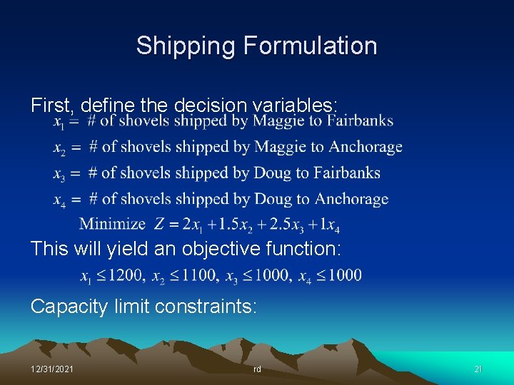
Shipping Formulation First, define the decision variables: This will yield an objective function: Capacity limit constraints: 12/31/2021 rd 21

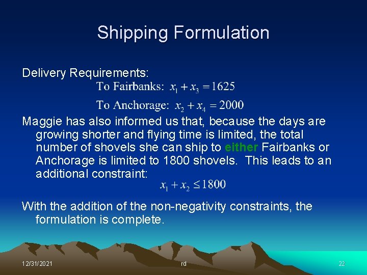
Shipping Formulation Delivery Requirements: Maggie has also informed us that, because the days are growing shorter and flying time is limited, the total number of shovels she can ship to either Fairbanks or Anchorage is limited to 1800 shovels. This leads to an additional constraint: With the addition of the non-negativity constraints, the formulation is complete. 12/31/2021 rd 22

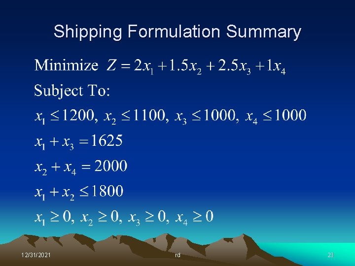
Shipping Formulation Summary 12/31/2021 rd 23

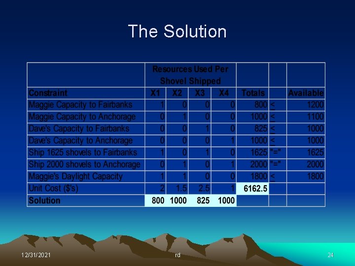
The Solution 12/31/2021 rd 24

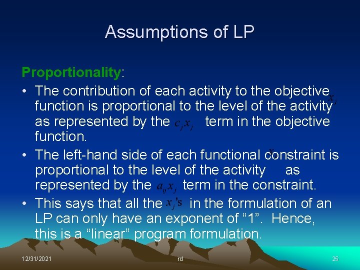
Assumptions of LP Proportionality: • The contribution of each activity to the objective function is proportional to the level of the activity as represented by the term in the objective function. • The left-hand side of each functional constraint is proportional to the level of the activity as represented by the term in the constraint. • This says that all the in the formulation of an LP can only have an exponent of “ 1”. Hence, this is a “linear” program formulation. 12/31/2021 rd 25

Assumptions (Cont. ) Additivity: Every function in a LP model (O. F. and L. H. S. of the constraints) is the sum of the individual contributions of the respective activities. Divisibility: All decision variables in an LP formulation are allowed to assume any value, including non-integer values, as long as all constraints are satisfied. Certainty: The value assigned to each parameter of a linear programming model is assumed to be a known constant. 12/31/2021 rd 26