Offset Free Tracking with MPC under Uncertainty Experimental

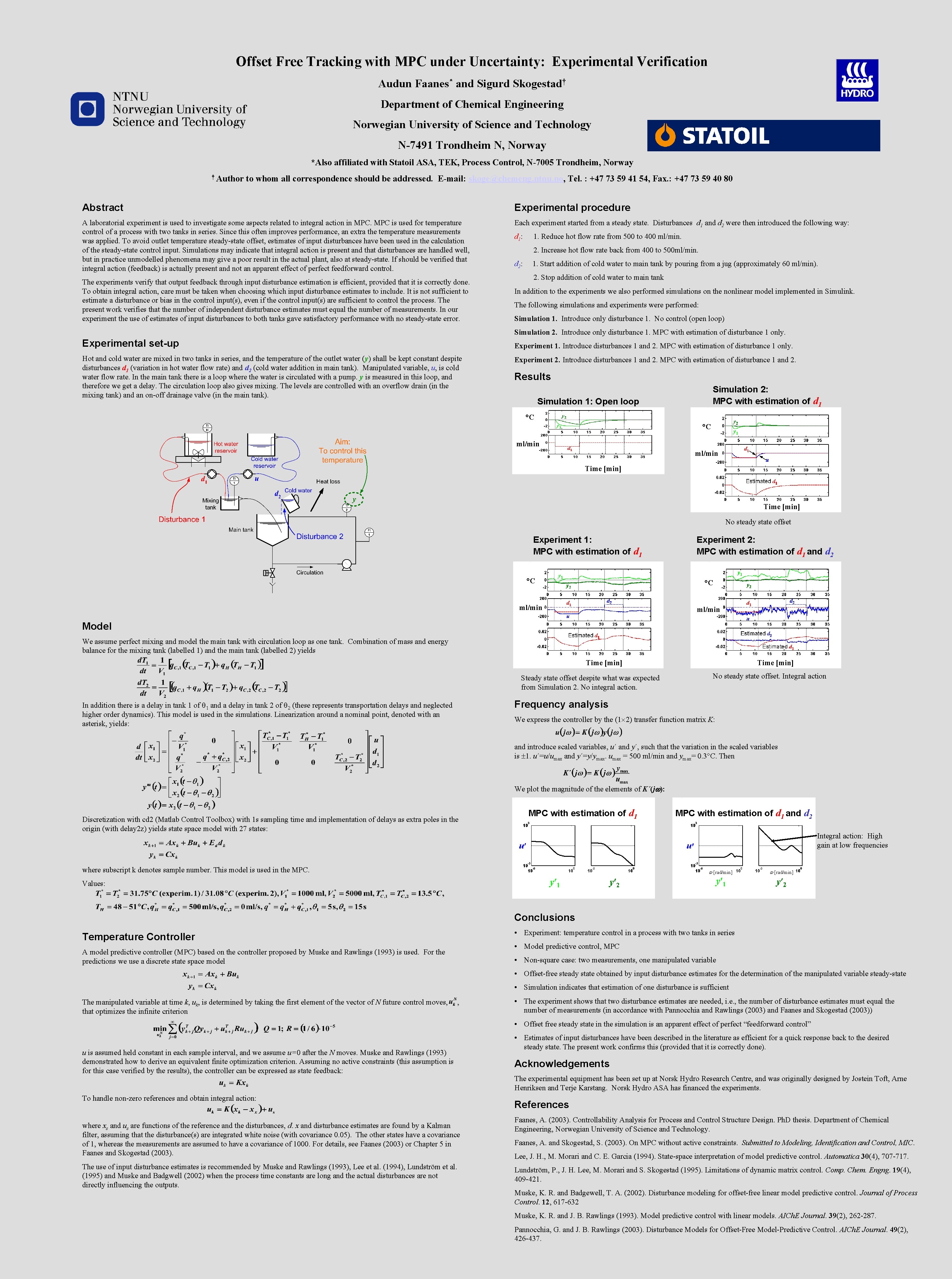
Offset Free Tracking with MPC under Uncertainty: Experimental Verification Audun Faanes* and Sigurd Skogestad† Department of Chemical Engineering Norwegian University of Science and Technology N-7491 Trondheim N, Norway *Also affiliated with Statoil ASA, TEK, Process Control, N-7005 Trondheim, Norway † Author to whom all correspondence should be addressed. E-mail: skoge@chemeng. ntnu. no, Tel. : +47 73 59 41 54, Fax. : +47 73 59 40 80 Abstract Experimental procedure A laboratorial experiment is used to investigate some aspects related to integral action in MPC is used for temperature control of a process with two tanks in series. Since this often improves performance, an extra the temperature measurements was applied. To avoid outlet temperature steady-state offset, estimates of input disturbances have been used in the calculation of the steady-state control input. Simulations may indicate that integral action is present and that disturbances are handled well, but in practice unmodelled phenomena may give a poor result in the actual plant, also at steady-state. If should be verified that integral action (feedback) is actually present and not an apparent effect of perfect feedforward control. Each experiment started from a steady state. Disturbances d 1 and d 2 were then introduced the following way: The experiments verify that output feedback through input disturbance estimation is efficient, provided that it is correctly done. To obtain integral action, care must be taken when choosing which input disturbance estimates to include. It is not sufficient to estimate a disturbance or bias in the control input(s), even if the control input(s) are sufficient to control the process. The present work verifies that the number of independent disturbance estimates must equal the number of measurements. In our experiment the use of estimates of input disturbances to both tanks gave satisfactory performance with no steady-state error. d 1: 1. Reduce hot flow rate from 500 to 400 ml/min. 2. Increase hot flow rate back from 400 to 500 ml/min. d 2: 1. Start addition of cold water to main tank by pouring from a jug (approximately 60 ml/min). 2. Stop addition of cold water to main tank In addition to the experiments we also performed simulations on the nonlinear model implemented in Simulink. The following simulations and experiments were performed: Simulation 1. Introduce only disturbance 1. No control (open loop) Simulation 2. Introduce only disturbance 1. MPC with estimation of disturbance 1 only. Experimental set-up Experiment 1. Introduce disturbances 1 and 2. MPC with estimation of disturbance 1 only. Hot and cold water are mixed in two tanks in series, and the temperature of the outlet water (y) shall be kept constant despite disturbances d 1 (variation in hot water flow rate) and d 2 (cold water addition in main tank). Manipulated variable, u, is cold water flow rate. In the main tank there is a loop where the water is circulated with a pump. y is measured in this loop, and therefore we get a delay. The circulation loop also gives mixing. The levels are controlled with an overflow drain (in the mixing tank) and an on-off drainage valve (in the main tank). Experiment 2. Introduce disturbances 1 and 2. MPC with estimation of disturbance 1 and 2. Results Simulation 2: MPC with estimation of d 1 Simulation 1: Open loop °C °C ml/min Time [min] No steady state offset Experiment 1: MPC with estimation of d 1 Experiment 2: MPC with estimation of d 1 and d 2 °C °C ml/min Model We assume perfect mixing and model the main tank with circulation loop as one tank. Combination of mass and energy balance for the mixing tank (labelled 1) and the main tank (labelled 2) yields Time [min] Steady state offset despite what was expected from Simulation 2. No integral action. No steady state offset. Integral action Frequency analysis In addition there is a delay in tank 1 of 1 and a delay in tank 2 of 2 (these represents transportation delays and neglected higher order dynamics). This model is used in the simulations. Linearization around a nominal point, denoted with an asterisk, yields: We express the controller by the (1 2) transfer function matrix K: and introduce scaled variables, u´ and y´, such that the variation in the scaled variables is 1. u´=u/umax and y´=y/ymax. umax = 500 ml/min and ymax= 0. 3°C. Then We plot the magnitude of the elements of K´(jw): Discretization with cd 2 (Matlab Control Toolbox) with 1 s sampling time and implementation of delays as extra poles in the origin (with delay 2 z) yields state space model with 27 states: MPC with estimation of d 1 and d 2 Integral action: High gain at low frequencies where subscript k denotes sample number. This model is used in the MPC. [rad/min] Values: Conclusions • Experiment: temperature control in a process with two tanks in series Temperature Controller • Model predictive control, MPC A model predictive controller (MPC) based on the controller proposed by Muske and Rawlings (1993) is used. For the predictions we use a discrete state space model • Non-square case: two measurements, one manipulated variable • Offset-free steady state obtained by input disturbance estimates for the determination of the manipulated variable steady-state • Simulation indicates that estimation of one disturbance is sufficient The manipulated variable at time k, uk, is determined by taking the first element of the vector of N future control moves, that optimizes the infinite criterion , • The experiment shows that two disturbance estimates are needed, i. e. , the number of disturbance estimates must equal the number of measurements (in accordance with Pannocchia and Rawlings (2003) and Faanes and Skogestad (2003)) • Offset free steady state in the simulation is an apparent effect of perfect “feedforward control” u is assumed held constant in each sample interval, and we assume u=0 after the N moves. Muske and Rawlings (1993) demonstrated how to derive an equivalent finite optimization criterion. Assuming no active constraints (this assumption is for this case verified by the results), the controller can be expressed as state feedback: To handle non-zero references and obtain integral action: where xs and us are functions of the reference and the disturbances, d. x and disturbance estimates are found by a Kalman filter, assuming that the disturbance(s) are integrated white noise (with covariance 0. 05). The other states have a covariance of 1, whereas the measurements are assumed to have a covariance of 1000. For details, see Faanes (2003) or Chapter 5 in Faanes and Skogestad (2003). The use of input disturbance estimates is recommended by Muske and Rawlings (1993), Lee et al. (1994), Lundström et al. (1995) and Muske and Badgwell (2002) when the process time constants are long and the actual disturbances are not directly influencing the outputs. • Estimates of input disturbances have been described in the literature as efficient for a quick response back to the desired steady state. The present work confirms this (provided that it is correctly done). Acknowledgements The experimental equipment has been set up at Norsk Hydro Research Centre, and was originally designed by Jostein Toft, Arne Henriksen and Terje Karstang. Norsk Hydro ASA has financed the experiments. References Faanes, A. (2003). Controllability Analysis for Process and Control Structure Design. Ph. D thesis. Department of Chemical Engineering, Norwegian University of Science and Technology. Faanes, A. and Skogestad, S. (2003). On MPC without active constraints. Submitted to Modeling, Identification and Control, MIC. Lee, J. H. , M. Morari and C. E. Garcia (1994). State-space interpretation of model predictive control. Automatica 30(4), 707 -717. Lundström, P. , J. H. Lee, M. Morari and S. Skogestad (1995). Limitations of dynamic matrix control. Comp. Chem. Engng. 19(4), 409 -421. Muske, K. R. and Badgewell, T. A. (2002). Disturbance modeling for offset-free linear model predictive control. Journal of Process Control. 12, 617 -632 Muske, K. R. and J. B. Rawlings (1993). Model predictive control with linear models. AICh. E Journal. 39(2), 262 -287. Pannocchia, G. and J. B. Rawlings (2003). Disturbance Models for Offset-Free Model-Predictive Control. AICh. E Journal. 49(2), 426 -437.