OCEAN OPTICS SCIENCE IN SUPPORT OF QUANTITATIVE IMAGING

OCEAN OPTICS SCIENCE IN SUPPORT OF QUANTITATIVE IMAGING OF COASTAL WATERS Dariusz Stramski Marine Physical Laboratory Scripps Institution of Oceanography University of California, San Diego COAST Meeting 29 – 30 September 2004 - OSU, Corvallis OR

R(l) = f [ IOPs(l) ] = f [ a(l), b. E(y, l), b. I(y, l’→ l) ] ≈ f [ bb(l) / ( a(l) + bb(l) ) ] ≈ f [ bb(l) / a(l) ] IOPs(l) = f [ seawater constituents ] R(l) = f [ seawater constituents ]

Seawater is a complex optical medium with a great variety of particle types and soluble species 10 mm

Three- or four-component model based on few broadly defined seawater constituents IOP(l) = IOPw(l) + IOPp(l) + IOPCDOM(l) IOPp(l) = IOPph(l) + IOPd(l) IOPd+CDOM(l) = IOPd(l) + IOPCDOM(l)

A three-component model of absorption

Chlorophyll-based models IOPph(l) = f [ Chl ] IOPp(l) = f [ Chl ] IOP(l) = IOPw(l) + f [ Chl ]

Case 1 and Case 2 Waters Morel and Prieur (1977); Gordon and Morel (1983)

• Average trends • Large, seemingly random, variability

Chlorophyll algorithms more than 30 years of history Clarke, Ewing and Lorenzen (1970)

Bricaud et al. (1998)

Beam attenuation vs chlorophyll Loisel and Morel (1998)

Standard Chl algorithms in the Baltic Sea Darecki and Stramski (2004)

Case 1/Case 2 bio-optics Stagnation New science strategy Reductionist approach

Reductionist reflectance / IOP model Ni

EXAMPLE CRITERIA • Manageable number of components • The sum of components should account for the total bulk IOPs as accurately as possible • The components should play a specific well-defined role in ocean optics, marine ecosystems, biogeochemistry, water quality, etc.

Example components of suspended particulate matter Living Particles Autotrophs 1. Picophytoplankton <2 mm 2. Small nanophytoplankton 2 -8 mm 3. Large nanophytoplankton 8 -20 mm 4. Microphytoplankton 20 -200 mm Heterotrophs 5. Bacteria ~0. 5 mm 6. Microzooplankton O(1 -100) mm s i ( l ) = Qi ( l ) G i Non-Living Particles Organic 7. Small colloids 0. 02 -0. 2 mm 8. Larger colloids 0. 2 -1 mm 9. Detritus >1 mm Inorganic 10. Colloidal/Clay minerals <2 mm 11. Larger (Silt/Sand) minerals >2 mm

Stramski et al. (2001)

Interspecies variability in absorption Stramski et al. (2001)

Interspecies variability in scattering Stramski et al. (2001)

Intraspecies variability over a diel cycle Thalassiosira pseudonana Stramski and Reynolds (1993)

Absorption of mineral particles Babin and Stramski (2004); Stramski et al. (2004)

Asian mineral dust Stramski and Wozniak (2004)

Scattering phase functions of bubbles Piskozub et al. (2004)

Reductionist reflectance / IOP model

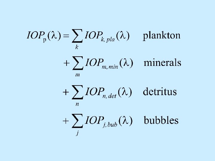
IOP model Stramski et al. (2001)

Size distribution

Absorption Scattering

Absorption Backscattering

Radiative transfer model Mobley and Stramski (1997)

The complexity of seawater as an optical medium should not deter us from pursuing the proper course in basic research to ensure quantitatively meaningful applications in coastal water imaging