Ocean Mixed Layer Dynamics and its Impact on

Ocean Mixed Layer Dynamics and its Impact on SST & Climate Variability Michael Alexander Earth System Research Lab michael. alexander@noaa. gov http: //www. cdc. noaa. gov/people/ michael. alexander/presentations

Ocean Mixed layer • • Turbulence creates a well mixed surface layer where temperature (T), salinity (S) and density (ρ) are nearly uniform with depth Primarily driven by vertical processes (assumed here) but can interact with 3 -D circulation • Density jump usually controlled by temperature but sometimes by salinity (especially in high latitudes) • Often “ measured” by the depth at which T is some value less than SST (e. g. ∆T = 0. 5) • Under goes large seasonal cycle • This impacts the evolution of ocean temperature anomalies and has important biological consequences surface T s ∆T ∆T=Tb-Tm ρ

Vertical Flux: Entrainment and MLD (h) Entrainment “To pull or draw along after itself” MLD – Mixed Layer Depth or h When deepening: dh/dt = we we = M + B – D / (D - S) Where M - Mechanical Turbulence (wind stirring) B - Buoyancy Forcing Net surface heating/cooling (Qnet) Precipitation – Evaporation (P-E) D - Dissipation (eh) Δρ Density jump at base of the ML S - Shear across ML (not in all models) When Shoaling: we = 0 (no detrainment, h reforms closer to the surface) h = M /(B – D)

Seasonal Cycle of Temp & MLD Northeast Pacific (50ºN, 145ºW) MLD (h)

Climatological Mixed Layer Depth (m)

SST Tendency Equation Integrated heat budget over the mixed layer: v – Tm – Tb – h – we – Qnet – Qswh – A – ρ – C – Variables velocity (current in ML) mixed layer temp (SST) temp just beneath ML mixed layer depth mean vertical velocity entrainment velocity net surface heat flux penetrating shortwave radiation horizontal eddy viscosity coefficient density of sea water Specific heat of sea water Qnet

Temperature change due to the surface heat flux • Over March through August a location in the North Pacific typically receives 150 Wm-2 flux through the surface. Assuming a constant mixed layer depth of 50 m, and no other changes in the ocean how much will the SST change over that time? • d. Tm/dt = d(SST)/dt = Qnet/ρch • ΔSST = (Qnet/ρch) x Δt • ρ = 1025 kg/m 3; c = 3850 Joules/(kg °C) • ΔSST = (150 Wm-2 / (1025 kg m-3 x 3850 Joules kg-1 °C-1 x 50 m)) * (184 days * 86400 s day-1) • SST = 12. 1°C • => Check units (W = J s-1) • => reasonable value for winter to summer change in SST

Surface Heat Flux Zonal Average Mean Standard Deviation Entrainment Flux

Observed Standard Deviation of SST Anomalies (°C) March August

Processes for Generating SST Anomalies

Simple model for generating SST variability “stochastic model” Heat fluxes associated with weather events, “random forcing” Ocean response to flux back heat which slowly damps SST anomalies F -λ Tm SST anomalies form Fixed depth ocean No currents Air-sea interface d. Tm/dt = Qnet ρch d. Tm/dt = F – λ Tm ρch Bottom

Stochastic SST Anomaly model II idealized forcing and time series Null Hypothesis for midlatitude SST variability

Stochastic Model: correspondence to the real world? Observed and Theoretical Spectra for SST anomalies (SSTA) at a location in the North Pacific Ocean Temperature Variance SSTA Variance No damping Atm forcing 10 yr 1 yr Spread (5%-95%) Observed Theoretical spectra (white line) of stochastic model 1 mo Period Atmospheric forcing and ocean feedback can be estimated from data. Then can then develop stochastic model and generate multiple time series to look at spread

Patterns of Surface Fluxes and SSTs: example North Atlantic Oscillation Contours are sea level pressure (SLP); vectors - winds Shading left is SST anomalies, on right is the Flux anomalies NAO north-south SLP anomaly pattern over the Atlantic

The Reemergence Mechanism Qnet’ • • • MLD • Winter Surface flux anomalies Create SST anomalies which spread over ML ML reforms close to surface in spring Summer SST anomalies strongly damped by air-sea interaction Temperature anomalies persist in summer thermocline Re-entrained into the ML in the following fall and winter Namias and Born 1970, 1974; Alexander and Deser (1995, JPO); Alexander et al. 1999 +

Reemergence in three North Pacific regions Regression between SST anomalies in April-May with monthly temperature anomalies as a function of depth. Regions Alexander et al. (1999, J. Climate)

Reemergence in the North Atlantic Reg 2 - Northeast Atlantic (47%) Reg 1 - Subtropical Atlantic (48%) Timlin, Alexander, Deser, 2002, J. Climate

Reemergence of SST Tripole Leading EOF of March SST Auto-correlation of EOF PC time series Reemergence of the SST North Atlantic tripole Level of significance ERSSTv 2 Datasets [1950 -2003] Degrees Celsius Watanabe and Kimoto (2000); Timlin et al. 2002, Deser et al 2003, De Coetlogon and Frankignoul 2003 : all in J. Climate

Impact of reemergence on SST Persistence: Augmenting the Stochastic SST model Entraining Model (EM) Obs (dashed) Heat content (EM) SST (OBS) Deser et al. 2003

North Atlantic Entraining Model (EM) Obs (dashed) Heat content (EM) SST (OBS) Deser et al. 2003 Heff = winter MLD for interannual variability in a stochastic model

Main Concepts • Mixed Layers – Processes that control its depth – Wind stirring buoyancy forcing, density jump at base of ML – Processes that control its temperature (SST) • Surface heat flux • Entrainment heat flux • Mechanisms for the behavior of SST anomalies • Stochastic model • Reemergence • Large scale patterns of atmospheric forcing organizes fluxes, shapes SST Anomaly and reemergence patterns • Questions?

1. What is the oceanic reemergence? 2. Surface signature of reemergence in the Labrador Sea Auto-correlation of the Labrador SST time series (Starting from March), e. g. for lag=1, March and April time series are correlated, for lag =2 March and May etc. Sea Surface Temperature e-folding = ~ 36 mths Level of significance ERSSTv 2 Datasets [1950 -2003] Degrees Celcius e-folding==~~44 mths e-folding Deser et al. 2003 (J. Clim) Reemergence of the late winter SST anomalies a year after Auto-correlation of the Labrador SST time series (all months considered), e. g. for lag=1, Jan 50/Feb 50/…/Dec 00 values are correlated with Feb 50/Mar 50/…/Jan 01 values

Atmosphere forcing the ocean in winter: NAO & the Atlantic SST tripole March SST EOF 1 (shade) Regressed JFM SLP (contour) PC time series: March SST (bars), JFM MSLP (line) Correlation=0. 63 NCEP MSLP [1950 -2003] e. g. Deser and Timlin (1997), J. Clim.

Summary • Forcing of SST (mixed layer temperature – Net heat flux key term, Ekman transport & entrainment also important – SST anomalies larger in summer than winer due to shallow MLD • Processes that impact extratropical SST variability – Stochastic atmospheric forcing – Reemergence • Atmospheric Bridge – Tropical Pacific => Global SSTs – Impacts in both winter and summer – Influence of air-sea feedback on extratropical atmosphere complex • Other Processes that influence SST variability – Cloud - SST feedbacks – Ocean currents & Rossby waves in western N. Pacific – Changes in the Thermohaline Circulation

Additional Topics • The flux components and their variability • Schematic of the mixed layer model • Pattern of atmospheric circulation (SLP) and the underlying fluxes) • Basin-wide reemergence • The Pacific Decadal Oscillation • Wind generated Rossby waves and its relation to SSTs • The Latif and Barnett mechanism for the PDO and “problems” with this mechanism

Atmosphere-Ocean Ice Model Atmospheric GCM – NCAR CAM 2–T 42 resolution Ice Thermodynamic portion of NCAR CSIMv 4 Ocean Mixed layer Model (MLM) • An individual column model with a uniform mixed layer • Atop a layered model that represents conditions in the pycnocline • Prognostic ML depth • Same grids as the atmosphere (128 lon x 64 lat) • 36 vertical levels (from 0 m to 1500 m depth) • • • higher resolution close to surface and a realistic bathymetry Flux correction needed to get reasonable climate Cassou et al. 2007 J Clim; Alexander et al. 2000 JGR, Alexander et al 2002 – J. Clim ; Gaspar 1988 – JPO

Mixed Layer Ocean Model Qnet Qcor Qwe Tm 1 Tb 1 Qswh CA h (MLD)

Mean ML Budget terms (Wm-2) in January From an AGCM couple to a mixed layer ocean model Surface Flux Qnet Ekman Qek = cvek( Tm) Entrainment Qwe = cwe(Tb-Tm)

Mean Mixed Layer Budget terms (Wm-2) in August

Standard Deviation of the Mixed Layer Budget Terms (Wm-2) in January

Standard Deviation of Fluxes in August Results from an AGCM- Ocean MLM Qnet W m-2 Qwe = cwe(Tb-Tm) W m-2 Qwe / Qnet

Wind Generated Rossby Waves L Atmosphere ML Ocean Thermocline West Rossby Waves East 1) After waves pass ocean currents adjust 2) Waves change thermocline depth, if mixed layer reaches that depth, cold water can be mixed to the surface

Observed Rossby Waves & SST Correlation Obs SST hindcast With thermocline depth anomaly KE Region: 40°N, 140°-170°E SSTOBS March SSTfcst T 400 Forecast equation for SST based on integrating wind stress (curl) forcing and constant propagation speed of the (1 st Baroclinic) Rossby wave Schneider and Miller 2001 (J. Climate)

Forecast Skill: Correlation with Obs SST Wave Model & Reemergence Wave Model Reemergence years Schneider and Miller 2001 (J. Climate)

Climatological heat fluxes August

Zonal Average of the standard deviation of the mixed layer budget terms

Observed SST ( C) / SLP (mb) Warm-Cold (5003) DJF JAS

Evolution of the leading pattern of SST variability as indicated by extended EOF analyses No ENSO; Reemergence Alexander et al. 2001, Prog. Ocean. ENSO; No Reemergence

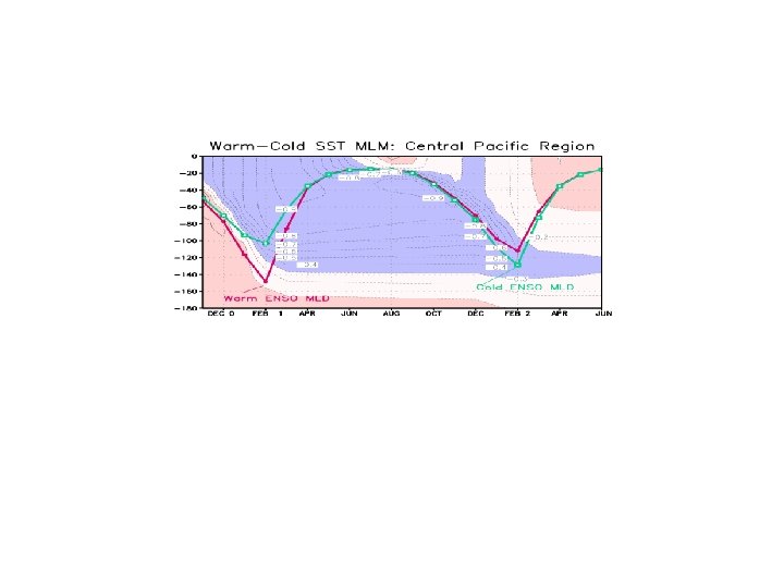
Upper Ocean: Temperature and mixed layer depth El Niño – La Niña model composite: Central North Pacific Alexander et al. 2002, J. Climate

ENSO SST & MLD in Western N. Pacific Region Niño – Niña: NCEP Ocean Temp & White MLD (1980 -2001) La Niña MLD °C El Niño MLD