Obtaining the Regression Line in R data healthread

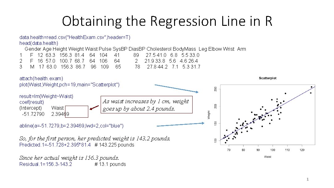
Obtaining the Regression Line in R data. health=read. csv("Health. Exam. csv", header=T) head(data. health) Gender Age Height Waist Pulse Sys. BP Dias. BP Cholesterol Body. Mass Leg Elbow Wrist Arm 1 F 12 63. 3 156. 3 81. 4 64 104 41 89 27. 5 41. 0 6. 8 5. 5 33. 0 2 F 16 57. 0 100. 7 68. 7 64 106 64 2 21. 9 33. 8 5. 6 4. 6 26. 4 3 M 17 63. 0 156. 3 86. 7 96 109 65 78 27. 8 44. 2 7. 1 5. 3 31. 7 attach(health. exam) plot(Waist, Weight, pch=19, main="Scatterplot") result=lm(Weight~Waist) coef(result) (Intercept) Waist -51. 72790 2. 39469 As waist increases by 1 cm, weight goes up by about 2. 4 pounds. abline(a=-51. 7279, b=2. 39469, lwd=2, col="blue") So, for the first person, her predicted weight is 143. 2 pounds. Predicted. 1=-51. 728+2. 395*81. 4 # 143. 225 pounds Since her actual weight is 156. 3 pounds. Residual. 1=156. 3 -143. 2 # 13. 1 pounds 1

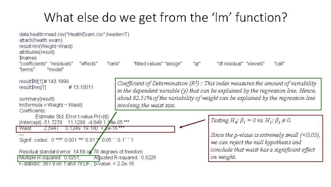
What else do we get from the ‘lm’ function? data. health=read. csv("Health. Exam. csv", header=T) attach(health. exam) result=lm(Weight~Waist) attributes(result) $names "coefficients" "residuals" "effects" "rank" "fitted. values" "assign" "terms" "model" result$fit[1] # 143. 1999 result$res[1] # 13. 10011 "qr" "df. residual" "xlevels" "call" Coefficient of Determination (R 2) : This index measures the amount of variability in the dependent variable (y) that can be explained by the regression line. Hence, about 82. 51% of the variability of weight can be explained by the regression line involving the waist size. summary(result) lm(formula = Weight ~ Waist) Coefficients: Estimate Std. Error t value Pr(>|t|) (Intercept) -51. 7279 11. 1288 -4. 648 1. 34 e-05 *** Waist 2. 3947 0. 1249 19. 180 < 2 e-16 *** --Signif. codes: 0 ‘***’ 0. 001 ‘**’ 0. 01 ‘*’ 0. 05 ‘. ’ 0. 1 ‘ ’ 1 Residual standard error: 14. 68 on 78 degrees of freedom Multiple R-squared: 0. 8251, Adjusted R-squared: 0. 8228 F-statistic: 367. 9 on 1 and 78 DF, p-value: < 2. 2 e-16 Testing H 0: β 1 = 0 vs. H 1: β 1 ≠ 0. Since the p-vlaue is extremely small (<0. 05), we can reject the null hypothesis and conclude that waist has a significant effect on weight.

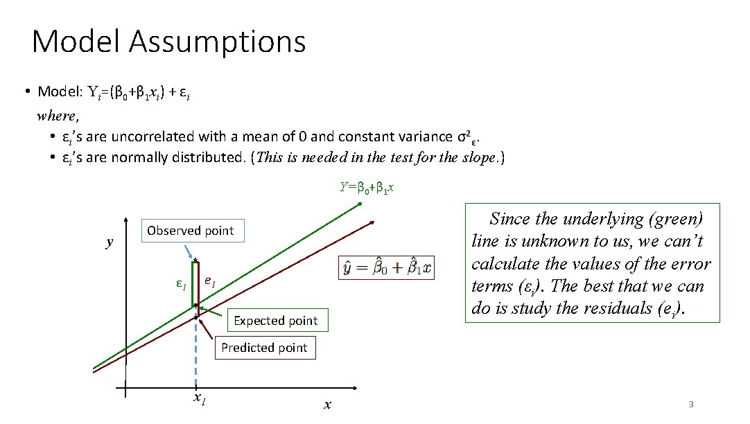
Model Assumptions • Model: Yi=(β 0+β 1 xi) + εi where, • εi’s are uncorrelated with a mean of 0 and constant variance σ2ε. • εi’s are normally distributed. (This is needed in the test for the slope. ) Y=β 0+β 1 x y Since the underlying (green) line is unknown to us, we can’t calculate the values of the error terms (εi). The best that we can do is study the residuals (ei). Observed point * ε 1 e 1 Expected point Predicted point x 1 x 3

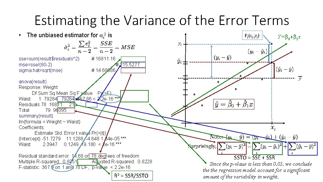
Estimating the Variance of the Error Terms • The unbiased estimator for σε 2 is Pi(xi, yi) Y=β 0+β 1 x yi sse=sum(result$residuals^2) mse=sse/(80 -2) sigma. hat=sqrt(mse) * # 16811. 16 * # 215. 5277 # 14. 68086 anova(result) Response: Weight Df Sum Sq Mean Sq F value Pr(>F) Waist 1 79284 367. 86 < 2. 2 e-16 *** Residuals 78 16811 216 Total 79 96095 summary(result) lm(formula = Weight ~ Waist) Coefficients: Estimate Std. Error t value Pr(>|t|) (Intercept) -51. 7279 11. 1288 -4. 648 1. 34 e-05 *** Waist 2. 3947 0. 1249 19. 180 < 2 e-16 *** Residual standard error: 14. 68 on 78 degrees of freedom Multiple R-squared: 0. 8251, Adjusted R-squared: 0. 8228 F-statistic: 367. 9 on 1 and 78 DF, p-value: < 2. 2 e-16 R 2 = SSR/SSTO * * * y * * * xi SSTO = SSE + SSR Since the p-vlaue is less than 0. 05, we conclude the regression model account for a significant 4 amount of the variability in weight.

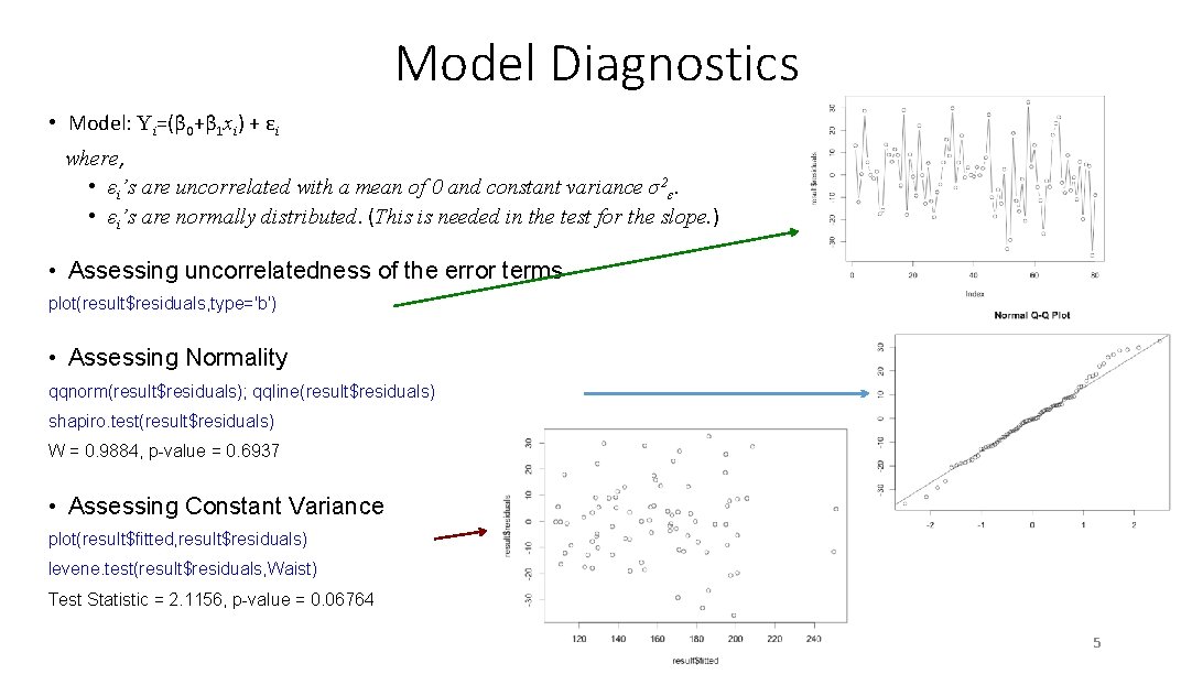
Model Diagnostics • Model: Yi=(β 0+β 1 xi) + εi where, • εi’s are uncorrelated with a mean of 0 and constant variance σ2ε. • εi’s are normally distributed. (This is needed in the test for the slope. ) • Assessing uncorrelatedness of the error terms plot(result$residuals, type='b') • Assessing Normality qqnorm(result$residuals); qqline(result$residuals) shapiro. test(result$residuals) W = 0. 9884, p-value = 0. 6937 • Assessing Constant Variance plot(result$fitted, result$residuals) levene. test(result$residuals, Waist) Test Statistic = 2. 1156, p-value = 0. 06764 5