Observations of stars Hyades open cluster Observations of

Observations of stars Hyades open cluster

Observations of stars

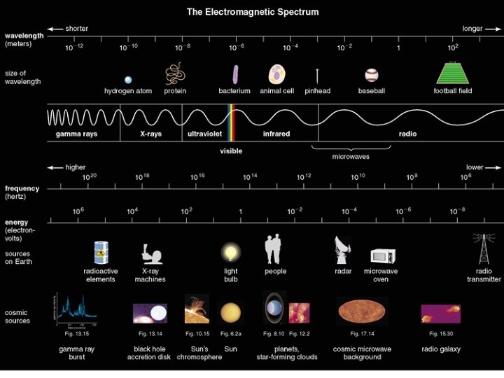
Astronomers count photons! We can measure three things about a photon: • What direction did it come from? • When did it arrive? • What was its energy (wavelength/color)?

Different types of observing modes 1. Count photons in a fixed region of the sky (aperture), a fixed window of time (exposure time), and a fixed wavelength range (filter or band). what we call “photometry” 2. Count photons as a function of direction in a fixed window of time (exposure time), and a fixed wavelength range (filter or band). what we call “imaging”

Different types of observing modes 3. Count photons as a function of wavelength in a fixed region of the sky (aperture), and a fixed window of time (exposure time). what we call “spectroscopy” 4. Count photons as a function of time in a fixed region of the sky (aperture), and a fixed wavelength range (filter or band). what we call “time series photometry”

Different types of observing modes 5. Count photons as a function of direction AND time in a fixed wavelength range (filter or band). what we call “time series imaging” 6. Count photons as a function of wavelength AND time in a fixed region of the sky (aperture). what we call “time series spectroscopy”

Different types of observing modes 7. Count photons as a function of direction AND wavelength in a fixed window of time (exposure time). what we call “integral field spectroscopy” 8. Count photons as a function of direction AND time AND wavelength. the holy grail of observational astronomy…
 f : luminosity/area (erg/s/cm 2)")
Luminosity and flux Luminosity Flux L : energy/time (erg/s) f : luminosity/area (erg/s/cm 2) Inverse square law:

Photometric filters

SDSS filters

Photometric Filters Astronomical fluxes are usually measured using filters The flux in the SDSS g filter is: The flux in the SDSS r filter is:
 has 100 x")
Apparent magnitude A star that is 5 magnitudes brighter (smaller m) has 100 x the flux.

Absolute magnitude M = apparent magnitude the star would have if it were 10 pc away. distance modulus

Hipparcos Data

Bolometric magnitudes M is measured in a band. To get the light from all wavelengths, we must add a correction. Bolometric correction: BC depends on band star spectrum. By definition, BC=0 for V-band T=6600 K

Color = crude, low resolution, estimate of spectral shape • distance independent • indicator of surface temperature • by definition, (B-V)=0 for Vega (T~9500 K)

Color • Measure a star’s brightness through two different filters V R B • Take the ratio of brightness: (redder filter)/(bluer filter) if ratio is large red star if ratio is small blue star e. g. , V/B
 The color of a star measured like this tells")
Color ↑↑ BV wavelength (nm) The color of a star measured like this tells us its temperature!

Stellar spectra The solar spectrum can be approximated as • a blackbody + • absorption lines (looking at hotter layers through cooler outer layers)
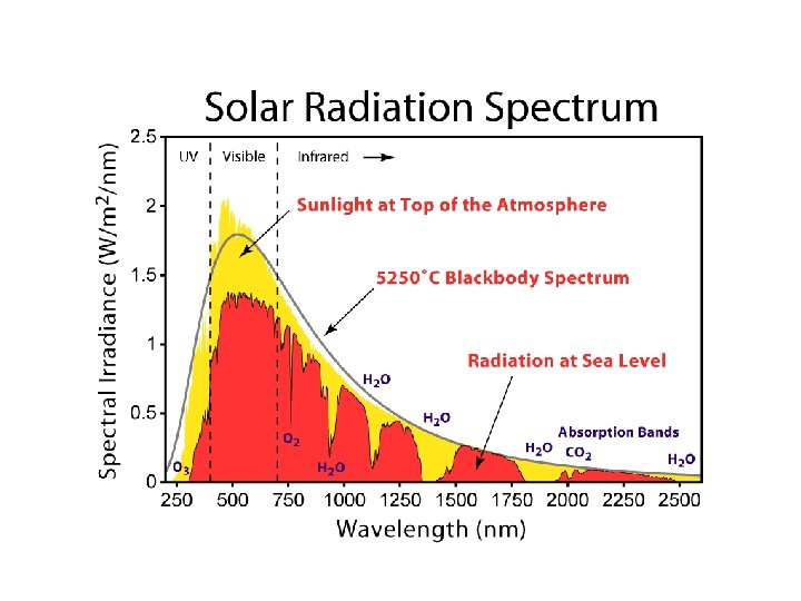

Blackbody radiation erg s-1 cm-2 Hz-1 st-1 • Effective temperature of a star = T of a blackbody that gives the same Luminosity per unit surface area of the star. Stefan–Boltzmann law For sun: Te = 5, 778 K

Blackbody Spectrum or thermal spectrum

Stellar spectra are not perfect blackbodies

Atomic energy levels • electrons orbit the nucleus in specific energy levels • electrons can jump between energy levels given the right energy

Emission of light ephoton atom

Absorption of light ephoton atom

Energy levels for Hydrogen Energy

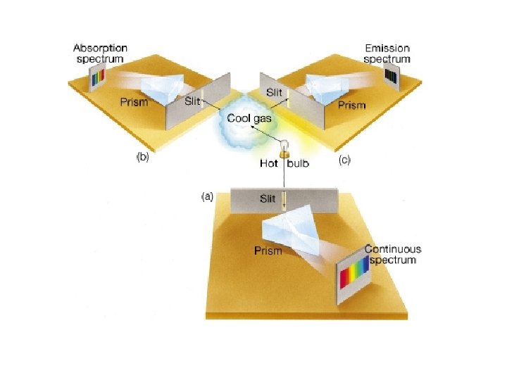
Visible spectrum shows signature of hydrogen atoms IR Visible UV Emission line spectrum Absorption line spectrum

Wavelength of light

Spectrum of Sun

Spectral lines Strength of lines depends on temperature. e. g. , Balmer lines: transitions from n=2 to higher states n=3 n=2 n=1 T < 5, 000 K: all Hydrogen is in ground (n=1) state no lines T > 20, 000 K: all Hydrogen is ionized no lines T ~ 10, 000 K: some Hydrogen is in n=2 state strong lines • Spectral lines are observational indicators of Te

Stellar spectra

Spectral lines Lines depend on temperature in stellar atmosphere + ionization potentials for relevant species e. g. , H He. II Ca. II Fe. I 13. 6 e. V 24. 6 e. V 54. 5 e. V 6. 1 e. V 11. 9 e. V 7. 9 e. V Ionization occurs when k. T ~ ionization potential/10

Spectral classification Te: 40 K 20 K 10 K 6. 7 K 5. 5 K 4. 5 K 3. 5 K early type late type

Spectral classification

Spectral classification

Spectral classification Oh Be A Fine Girl/Guy Kiss Me Omnivorous Butchers Always Find Good Kangaroo Meat Only Bored Astronomers Find Gratification Knowing Mnemonics

Luminosity class Stars of same type have different line widths wavelength Same T, different R different surface gravity g different surface pressure P Pressure broadening: orbitals of atoms are perturbed due to collisions broadening of spectral lines. Since , changes in R at fixed T are changes in L Spectral line widths luminosity classification Ia Ib Supergiants II Luminous giants III IV V VI VII Giants Subgiants Dwarfs Subdwarfs White dwarfs

Luminosity class

Special stars C: carbon stars - same Teff as K, M stars, but higher abundance of C than O all O goes to form CO. Remaining C forms C 2, CN. S: same Teff as K, M stars, but have extra heavy elements W: Wolf-Rayet - He in atmosphere instead of H, strong winds L: cooler than M stars. Some do not have fusion. T: cool brown dwarfs (700 -1, 000 K). Methane lines are prominent. The Sun is a G 2 V star
 diagram")
The first Hertzsprung-Russell (H-R) diagram

Hipparcos Color-Magnitude Diagram

Hipparcos Color-Magnitude Diagram

Plot luminosity vs. temperature high Luminosity low blue red Temperature

Understanding the H-R diagram high A Luminosity B low blue red Temperature

Understanding the H-R diagram high A C Luminosity low blue red Temperature

Understanding the H-R diagram high C Luminosity D low blue red Temperature

Understanding the H-R diagram high A C B D Luminosity low blue red Temperature

Understanding the H-R diagram high Luminosity low hot, big luminous cool, huge luminous sun hot, tiny faint blue cool, small faint red Temperature

Hipparcos H-R diagram

Theoretical H-R diagram
 nucleosynthesis: protons fuse to form He and heavier elements")
Chemical composition Primordial (Big Bang) nucleosynthesis: protons fuse to form He and heavier elements 3 minutes after the Big Bang. Ends 20 minutes later. Alpher, Bethe & Gammow, Physical Review L, 1948 75% H 25% He 0. 01% D Subsequent fusion inside massive stars and enrichment of the inter-stellar medium via supernovae, leads to future generations of stars with more heavy elements.

Stellar populations in the Milky Way

Stellar populations in the Milky Way Pop III Spatial Distribution Disk, |z|<200 pc Halo/spheroid Have not been found Kinematics (coherent) Disk rotation (220 km/s) No rotation Kinematics (dispersion) ~30 km/s large Metallicity Z~0. 02 Z<0. 01 Z~0 Age Young Old Primordial

Determining stellar properties Physical parameters: Measurements: • distance d • position on sky • luminosity L • flux in different bands • temperature Te • spectrum • radius R • time dependence of above • mass M • age t • chemical composition Xi

Determining distance Standard candle Standard ruler
")
Determining distance: Parallax RULER Define new distance unit: parsec (parallax-second)

Determining distance: Parallax
")
Determining distance: Parallax Point spread function (PSF)

Determining distance: Parallax Need high angular precision to probe far away stars. Error propagation: At what distance do we get a given fractional distance error?

Determining distance: Parallax e. g. , to get 10% distance errors Mission Dates Earth telescope HST Hipparcos 1989 -1993 Gaia 2013 -2018 SIM cancelled

Determining distance: moving cluster method Proper motion

Determining distance: secular parallax • Parallax method is limited by 2 AU baseline of earth’s orbit • Sun moves ~4 AU/yr toward Vega relative to local rotation of Galactic disk • Over a few years, this can build up to a large baseline • Unfortunately, other stars are not at rest, rather have unknown motions • However, if we average over many stars, their mean motion should be zero (relative to local rotation) • Can therefore get the mean distance to a set of stars

Determining distance: secular parallax RULER

Determining distance: moving cluster method RULER 1. 2. 3. 4. 5. 6. Measure proper motions of stars in a cluster Obtain convergent point Measure angle between cluster and convergent point Measure radial velocity of cluster Compute tangential velocity Use proper motion of cluster to get distance
 CANDLE For pulsating stars, SN, novae, measure flux")
Determining distance: Baade-Wesselink (moving stellar atmosphere) CANDLE For pulsating stars, SN, novae, measure flux and effective temperature at two epochs, as well as the radial velocity and time between the epochs. Solve for R 1 and R 2. R and T L d

Determining distance: spectroscopic parallax CANDLE • Stellar spectra alone can give us the luminosity class + spectral class position on HR diagram • This gives the absolute magnitude, which gives the distance modulus. • Basically, compare a star’s spectrum to an identical spectrum of another star with known luminosity. • This method is poor in accuracy (+/- 1 magnitude error in absolute magnitude 50% error in distance) • But it can be applied to all stars

Determining distance: main sequence fitting CANDLE • Measure the colors and magnitudes of stars in a cluster (e. g. , r and g-r) • Plot the HR diagram: r vs. g-r • Compare the HR diagram of another cluster of known distance: Mr vs. g-r • Find the vertical offset in HR diagram between the main sequences of the two clusters distance modulus

Determining distance: main sequence fitting CANDLE Hyades: d=47 pc Pleiades: d=136 pc

Determining distance: variable stars Cepheid variables: Pop I giants, M ~ 5 -20 Msun Pulsation due to feedback loop: An increase in T He. III (doubly ionized He) high opacity radiation can’t escape even higher T and P atmosphere expands low T He. II (singly ionized He) low opacity atmosphere contracts rinse and repeat…

Determining distance: variable stars RR-Lyrae variables: Pop II dwarfs, M ~ 0. 5 Msun

Determining distance: variable stars CANDLE Variable stars have a tight period-luminosity relation • Measure lightcurves: flux(t) • Get period P • From P-L relation, get L • Use L to get distance Very powerful method. Cepheids can be seen very far away. Used to measure H 0 P-L relation is calibrated on local variables with parallax measurements

Determining distance: dynamical parallax RULER For binary star systems on main sequence • Measure: period of orbit P, angular separation , fluxes f 1 and f 2 • Kepler’s 3 rd law: • Assume • Use Kepler to get • Use and to get preliminary distance • Use distance and fluxes to get luminosities L 1, L 2 • Use mass-luminosity relation for main sequence to get better masses • Iterate until convergence

Determining Luminosity 1. Measure flux or magnitude Measure distance 2. Measure spectrum line ratios and widths (i. e. , compare the star to a star of identical spectrum that has a known L)
 3. Blackbody")
Determining Temperature 1. Spectral lines spectral type 2. Colors (cheap and accurate) 3. Blackbody fitting or Wien’s law: (not good for very hot or cool stars) 4. Stellar atmosphere modeling (uncertain) 5. Measure angular size and flux (need very high resolution imaging)

Determining Radius • Very difficult because angular sizes are tiny. • Important because of: The sun at 1 pc distance has an angular radius of ~0. 5 mas • surface gravity • density • Temperature • testing models

Determining Radius: Interferometry yields high resolution images 1. Speckle interferometry ~ 0. 02 as Diffraction limited: e. g. , for HST (DT=2. 4 m), =0. 05 as

Determining Radius: Interferometry 2. Phase interferometry ~ 0. 01 as Fringes disappear when 3. Intensity Interferometry Hanbury-Brown and Twiss effect ~ 0. 5 mas The sun’s radius could be measured out to ~1 -10 pc
 • Lunar Occultation")
Determining Radius • Luminosity + Temperature Radius • Baade-Wesselink (moving atmosphere) • Lunar Occultation As a star disappears behind the moon, a Fresnel diffraction pattern is created that depends slightly on ~ 2 mas, only good for stars in ecliptic.

Determining radius: eclipsing binaries

Determining radius: eclipsing binaries

Determining Mass Only possible to measure accurately for binaries. Kepler’s 3 rd law: For Sun-Earth system:

Determining Mass: visual binaries

Determining Mass: visual binaries Visual binaries are binaries where the angular separation is detectable and the orbit can be traced out. • Find the center of mass of the system (c. o. m. must move with constant velocity) • Measure the period, semi-major angular separation and distance. • Solve for individual masses. Very sensitive to distance errors: • If distance is not known, radial velocity data is sufficient to get e. g. , for a circular orbit:

Determining Mass: visual binaries If the orbit is inclined, then we must know the inclination angle Don’t need i Need i In an inclined orbit, the center of mass does not lie at the ellipse focus. Find the projection that fixes this cos i

Determining Mass: spectroscopic binaries Spectroscopic binaries are unresolved binaries that are only detected via doppler shifts in their spectrum. • Single line binaries: single set of shifting spectral lines • Double line binaries: two sets of spectral lines (one from each star) • Two sets of lines, but for different spectral types

Determining mass: spectroscopic binaries

Determining Mass: spectroscopic binaries • Measure velocities and period • Can get a lower limit on M 1+M 2 since sin i <1

Determining Mass: spectroscopic binaries Need to measure both radial velocities - only possible with double line binaries. Need to know sin i. This is possible when: • also an eclipsing binary: sin i = 1 • also a visual binary: measure orbit • compute M 1+M 2 for a statistical sample where <sin 3 i> is known (For an isotropic distribution, <sin 3 i>=0. 42. However, no Doppler shift will be observed if i=0, so there is a selection effect that favors high inclinations)

Determining Mass: surface gravity • Pressure broadening of spectral lines surface gravity • Measure radius R • Sensitive to errors in R

Determining Mass: Gravitational lensing

Gravitational lensing

Determining Mass: Gravitational lensing

Determining Mass: gravitational microlensing Case of lensing when multiple images are unresolved and we only detect an increase in the flux of one image General Relativity: source lens Can compute the amplification of light due to multiple images image

Determining mass: gravitational microlensing

Determining mass: gravitational microlensing

Determining mass: gravitational microlensing

Determining Chemical Composition Theoretical: fractional abundances by mass X: Hydrogen Y: Helium Z: metals Sun: (0. 7, 0. 28, 0. 02) Observational: number density relative to Hydrogen, normalized to sun. e. g. , iron abundance So, for solar abundance: In our galaxy, , 10 times more iron: ranges from -4. 5 to +1. Need high resolution spectra + stellar atmosphere models to get abundances via fitting.

Hipparcos stars Determining age: Main Sequence turn-off The lack of blue dwarfs tells us that the age of M 6 is sufficiently old that the massive blue stars have died. M 6 cluster Yellow and red stars are still present because they live longer lives.
 at")
Determining age: Main Sequence turn-off • All stars arrived on the mainsequence (MS) at about the same time. • The massive stars on the top left of MS are the first to go. • The cluster is as old as the most luminous star that remains on the MS. • The position of the hottest, brightest star on a cluster’s MS is called the main-sequence turnoff point.

Determining age: Main Sequence turn-off A Which cluster is oldest? C B

Determining age: Isochrone Fitting Metallicity 63 million years 16 billion years 1 billion years

Determining age: Isochrone Fitting Open clusters 1. 4 billion years 2. 6 billion years

Determining age: Isochrone Fitting 6, 7, 8 billion years NGC 188: 7 billion years

Determining age: Isochrone Fitting 47 Tuc: 12 billion years

Determining age: Isochrone Fitting M 55: 12. 5 billion years

Determining age: Isochrone Fitting M 5: 13 -14 billion years

Determining age: Isochrone Fitting Measurement Errors • errors in brightness/colors • errors in distance/luminosity • errors in cluster membership Theoretical Errors • uncertain chemical abundances • uncertain amount of dust • uncertain stellar physics Typical error < 1 billion years
- Slides: 110